One frequent question I hear from SVS customers is whether whole exome sequence data can be used for principal components analysis (PCA) and other applications in population genetics. The answer is, “yes, but you need to be cautious.” What does cautious mean? Let’s take a look at the 1000 Genomes project for some examples.
Phase 3 of the 1000 Genomes Project was released in 2014. The latest major update to the autosomal data, version 5, was released in September. This iteration of the 1000 Genomes Project (1kGP) includes whole-genome sequence data for over 2500 individuals from 26 distinct worldwide populations. As a nice bonus, there is also a large amount of GWAS chip data available. Almost all of the samples have data for the Affymetrix SNP6.0 (Affy6) platform, and many of them also have Illumina 2.5M data. The chip data gives us a nice baseline for comparing methods and results in SVS.
For this analysis, I reduced the 1kGP data to exon regions only. I downloaded the 1kGP autosomal VCF files, used the UCSC browser to create a BED file of RefSeq exon regions (+/- 5 bp), then filtered the files and combined them using VCFtools. The resulting VCF file, containing about 2.2M variants, was imported to SVS for analysis.
Preparing the Data
SVS has methods for PCA, relatedness estimation, fixation indices, inbreeding estimation and other population-level statistics that are designed for use with data from GWAS chips. But even with GWAS data, we don’t usually use all available SNPs to run these statistics. It is usually best to reduce the data to a set of highly-informative markers. Generally speaking, informative markers will have high call rates, high minor allele frequencies (MAF), and will mostly be independent of one another (low pairwise linkage disequilibrium, or LD).
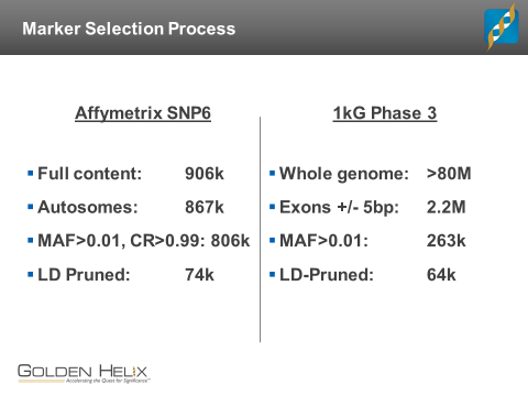
When working with exome data in SVS, it is usually possible to identify a set of informative variants to use for population statistics. One of the most important things is that your variant calls were processed and/or imported in such a way that genotype calls are present for homozygous-reference genotype calls. In that scenario, the software will treat the data no differently than genotypes from a GWAS chip, and you can proceed to select a set of informative SNPs. The following slide summarizes such a process for the 1kGP exome data as compared with the corresponding Affy6 genotypes:
Both datasets were filtered to include only SNPs with a minor allele frequency greater than 1%, with a maximum pair-wise LD R-squared of 10% within a 50-SNP window. The two processes returned similar-sized SNP lists: about 74k from Affy6 and 64k from the exomes. But there is minimal overlap in content here. Only 1011 of the Affy6 SNPs even fall within the same regions (exons +/-5bp) that the exome variants are drawn from. The Affy6 SNPs have an average MAF of 0.118; the average MAF in the exomes is 0.068. The median spacing between the Affy6 SNPs is 15kb; the median spacing of the exome variants is 3.8 kb. The exome variants are certain to be under different selective pressures than the broadly-distributed Affy6 SNPs.
PCA Results
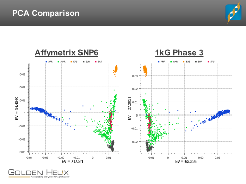
I used SVS to perform PCA on both datasets to find out if we get similar results from these two very different variant sets. The results were striking. The first two principal components, which broadly capture the continental-level stratification of the 1kGP samples, were essentially identical. As shown in the figure below, the only noticeable difference is that the first component is merely reflected around zero. This would make no practical difference if, for example, you were using the principal components as a correction factor in an association test. Further comparisons show that the first four components of the two variant sets are very similar, but diverge beginning with the fifth component. Beyond that point, PCA is generally detecting different features of the data. So you can use PCA to identify population stratification, but you need to be cautious about how you interpret the results.
What about relatedness testing?
Another common application for population-based data is relatedness testing. I ran the two variant sets through the SVS Identity-by-Descent (IBD) algorithm to see if there were any related samples in the 1kGP phase 3 data.
We must be careful about the structure of the population in this analysis. For the IBD method to give uniform results, the subjects need to come from a homogeneous population. The IBD algorithm is based on observed-versus-expected allele sharing, and the expected sharing rate for each SNP is based on that SNP’s observed MAF.
If subjects are drawn from two ethnic groups, and one group is much larger than the other, the majority group will establish the expected sharing rate. A common result of this is that the minority group will appear to have excess sharing at a large number of loci with “rare” minor alleles, and will have inflated IBD estimates as a result. This is especially problematic when the minority group is from a population that is not well represented in HapMap and other diversity catalogs. I first noticed this several years ago in a GWAS that included several Native Americans in addition to the Caucasian majority. The Native Americans were all unrelated, but had pair-wise IBD estimates indicating that they were all inter-related at the level of 2nd-3rd degree relatives. The 1kGP data has similar effects, but with much more diversity in the data.
I ran the IBD algorithm on the same two variant sets that were used for PCA. As expected, the ethnic diversity creates noise that makes it difficult to distinguish between more distant relationships, but the Affy6 and exome data agree that there appear to be 12 first-degree relative pairs in the 1kGP phase 3 version 5 data. The release notes indicate the removal of related samples in a previous version, but I think that they missed a few. Consider the following table:
| Sample1 | Sample2 | Population | SuperPop | IBD (Exome) | IBD (Affy6) | Relationship |
| NA20891 | NA20900 | GIH | SAS | 0.531 | 0.542 | Parent-Child |
| NA20882 | NA20900 | GIH | SAS | 0.545 | 0.539 | Parent-Child |
| HG03733 | HG03899 | STU | SAS | 0.587 | 0.571 | Full Sib |
| HG03873 | HG03998 | ITU – STU | SAS | 0.572 | 0.564 | Full Sib |
| HG03750 | HG03754 | STU | SAS | 0.557 | 0.544 | Parent-Child |
| NA19904 | NA19913 | ASW | AFR | 0.500 | 0.500 | Parent-Child |
| NA20317 | NA20318 | ASW | AFR | 0.500 | 0.500 | Parent-Child |
| NA20320 | NA20321 | ASW | AFR | 0.500 | 0.500 | Parent-Child |
| NA20334 | NA20355 | ASW | AFR | 0.500 | 0.500 | Parent-Child |
| NA20359 | NA20362 | ASW | AFR | 0.500 | 0.500 | Parent-Child |
| HG02429 | HG02479 | ACB | AFR | 0.492 | 0.483 | Full Sib |
| NA19331 | NA19334 | LWK | AFR | 0.424 | 0.439 | Full Sib |
IBD estimates of about 0.5 indicate a first-degree relationship. The values in the table range from 0.424 to 0.587. The values are a little bit noisy due to the multiple ethnic groups, but I’m quite certain of the relationships. I re-ran the analysis separately only the SAS (South Asian) and AFR (African) super-populations, and the results within the groups were much cleaner and confirmed this result.
The IBD algorithm also gives the probability of sample pairs sharing 0, 1 or 2 alleles IBD genome-wide, which can be used to infer the type of relationship. Parent-offspring pairs should have 100% sharing of 1 allele, and no sharing of 0 or 2 alleles. Sibling pairs should share 25%, 50%, and 25% respectively for 0, 1 and 2 copies. Based on this data (not shown), we can determine the types of relationships observed. Two results stand out to me:
- Samples NA20882, NA20891 and NA20900 form a family trio.
- Samples HG03873 and HG03998 appear to be siblings, but are reported to be from different populations. One is reported to be Indian Telegu (ITU), and the other Sri Lankan Tamil (STU). I reviewed the principal components to see if one of the pair might be mislabeled, but the ITU and STU groups are very similar in the PCA results, even when the South Asian populations are examined alone.
Final Thoughts
The SVS software doesn’t distinguish between sequence variants and chip-based genotypes for most genotype analysis functions. As such, exome variant data can be used for many GWAS-style analysis procedures. But be aware that exome data is distributed very differently than are the SNPs from GWAS chips, and you need to be cautious about interpreting the results.


