A recent email from a user of SVS:

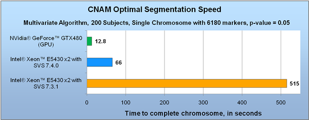
“Your CNAM Optimal Segmentation algorithm is by far the best I ever used and believe me, I’ve tried many. Great use of the GPU for segmentation – it is 3x faster than using my 8 CPUs alone and 25x faster compared to 1 CPU.”

SNP & Variation Suite (SVS) version 7.4 introduced an impressive array of new features that were not available in previous versions.  New features range from major items like the all-new Sequence Analysis Module to new shortcut keys and subtle improvements in infrastructure that most users will never notice.  We created a list of over 50 new or updated features, but even that list is not complete and does not capture the extent of the work performed by our development team.  I applaud them for their efforts.  Today, I’d like to specifically review some of the new and updated features for copy number analysis that are present in version 7.4.

Accelerated Segmentation
Here at Golden Helix headquarters, we refer to the Copy Number Analysis Module as CNAM (pronounced “see-nam”).  People often ask us if the CNAM CNV identification method is based on common methods like hidden Markov models or circular binary segmentation, and the answer is neither one.  CNAM uses a change-point identification algorithm based on the work of Dr. Douglas Hawkins [1,2,3,4].  It is a very powerful algorithm for accurately identifying changes in sequential data like genome-wide log ratio signals with the primary drawback being that it can be a little slow for large datasets.

That brings us to the first major CNAM improvement in version 7.4: GPU acceleration.  Software Engineer, Mike Thiesen, summarized this feature very nicely in an earlier blog entry while it was still in development.  By harnessing the power of modern computer graphics cards, SVS users are able to get a speed increase of 20 times or more for univariate segmentation.  Segmentation jobs that previously required several weeks can now be finished in a matter of days or hours.  If you need to repeat the job with different parameters, you can now do so without substantial impact on your overall analysis timeline.

Just as exciting as the acceleration of univariate segmentation is the acceleration we have achieved for multivariate segmentation, which was still in development at the time of Mike’s blog post.  In past versions, multivariate segmentation was simply not practical for large whole-genome analysis projects because of the time it required.  Now, in some of our test cases, it is even faster than univariate.  In SVS 7.4, we were able to make optimizations to the algorithm to speed up it substantially for CPU processing, and it is even faster with GPU acceleration.

Speed increase for multivariate segmentation in SVS 7.4. A major acceleration is achieved for CPU processing time in this version, and GPU acceleration makes it faster still.

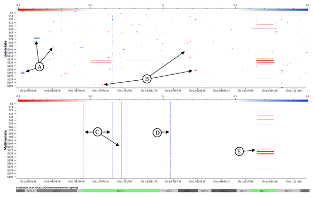
The CNAM multivariate segmentation tool is the only CNV identification tool I’m aware of that simultaneously considers the data from multiple subjects.  This feature makes it possible to accurately identify common CNVs (even very small ones), which is often cited as a major difficulty in CNV analysis.  As I explained in a previous entry, common CNVs are difficult to correctly identify because of the variable signal coming from the reference data used in log ratio (LR) calculations.  Because the reference signal doesn’t necessarily equate to two copies, the log ratio values in a common CNV region don’t follow the same patterns you see for rare CNVs.  If the average copy number for a common indel is between 1 and 2 in the reference group, then the study subjects with 2 copies will have an LR slightly above the baseline of 0 and subjects with 1 copy will have an LR slightly below the baseline of zero.  When considering one sample at a time, these slight variations are not always distinguishable from the flanking regions, and most segmentation algorithms fail to identify them correctly, especially when the CNV is covered by a small number of markers.

By simultaneously analyzing the data for all samples, we are able to identify the loci where many subjects have a minor distortion that may indicate a common polymorphic CNV.  Multivariate segmentation assigns the same set of segment endpoints to every subject and returns the average intensity for each subject within each segment.  A heatmap of these results shows wide regions of minimal variation interspersed with small, highly-variable segments.  The distribution of each segment will usually cluster into 2-3 groups, indicating unique copy number classes.  Watch for a new tutorial to be released soon with more information about using multivariate segmentation.

This figure illustrates the differences between univariate and multivariate segmentation. The upper panel shows univariate segmentation results, and the lower panel shows multivariate segmentation results. Red segments are probable deletions, while the blue segments are probable copy gains. (A-B) Rare copy gains and deletions detected only by univariate segmentation. (C) Small, common CNVs detected poorly by the univariate method, but with a better resolution by the multivariate method. (D) This common CNV was ignored as an outlier by univariate segmentation, which considers only one subject at a time because it is covered by only one marker. Multivariate segmentation, which simultaneously considers all subjects, was able to recognize that this single marker clearly has multiple copy states. (E) Large, common deletion that was accurately detected by both segmentation methods. The multivariate method provides better resolution of the segment endpoints.

The CNAM Window

The CNAM Optimal Segmenting window in SVS 7.4.

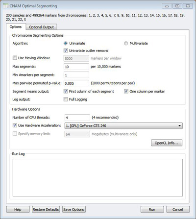
Experienced users of CNAM will notice that the segmentation dialog has changed a little bit.  The biggest difference is a new box called “Hardware Options.”  This contains the previously available option to specify the number of CPU threads to use, together with the new feature of auto-detecting the number of threads available.  It also contains the new “Use Hardware Acceleration” option, which controls the GPU acceleration features.  Any device that is compatible with the OpenCL standard should appear in this window.  Lists of compatible Nvidia and ATI devices can be found online.  If you think that your graphics card is supported, but it is not visible in the CNAM window, try updating the driver.

A more subtle change in the CNAM window is the control for the maximum number of segments per window.  The default behavior in the past was to use a moving window in segmentation to get increased efficiency.  We think the results are a little better when you don’t use a moving window, and GPU acceleration makes this approach more practical.  In the previous version, the maximum number of segments specified would be applied to every window, whether the window is a full chromosome or a sliding window of 5,000 markers. There is a penalty in the CNAM segmentation algorithm if the maximum number of segments is set too high, which presents us with a conundrum when we don’t use a moving window. Because we don’t really expect chromosome 1 to have the same number of CNVs as chromosome 21, we decided to make this parameter dynamic, and base it on the number of markers in a given chromosome. You are now asked to enter the maximum number of segments per 10,000 markers. The default value of 10 seems to work pretty well for data from most of the SNP platforms. If you have really high-density data, or the log gives you warnings about finding too many segments, you may want to increase this value.

Improved Affymetrix CEL File Import

The updated Affymetrix CEL file import window in SVS 7.4.

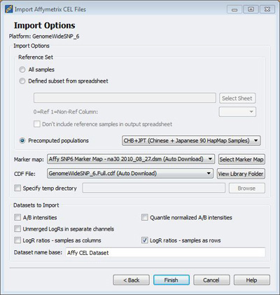
Affymetrix users will be pleased to know that we’ve updated and streamlined the process for importing copy number data from CEL files. In previous versions, you had to manually download Affymetrix library and map files and create a spreadsheet to indicate the reference status for each sample. In version 7.4, the software reads the CEL files to detect the platform you are using (250K Nsp, SNP Array 6.0, etc.) and automatically downloads library and map files (if you don’t already have them available). We have also introduced the option to use all samples as a pooled reference for LR calculations without having to create a reference status spreadsheet. Finally, you can now choose an option to download pre-computed reference data based on HapMap populations. This option should be attractive to researchers working with small sample sizes or who want to have consistent reference data across multiple projects.

We sometimes encounter confusion about how the reference data is used. The average intensity of the reference subjects is used as the expected intensity at each marker. This value becomes the denominator of the “ratio” in “log ratio,” which is calculated as log2(observed intensity/reference intensity). The reference subjects are not given any special attention in the quantile normalization process.

If you happen to prefer Illumina, Agilent, or Nimblegen, you will find that we have updated our import tools for those products as well.

Quality Assurance Menu
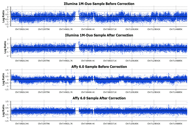
The Quality Assurance menu in SVS 7.4 includes a new CNV sub-menu with three procedures for CNV QA. Two of these items, “Percentile Based Winsorizing” and “Derivative Log Ratio Spread” (DLRS), were previously available as add-on scripts but are now included in the SVS standard package. The third item, “Wave Detection/Correction,” is brand new, and we are very excited about it. We have incorporated the Diskin [5] method for measuring genomic wave effects and correcting waves based on GC content. We strongly recommend using wave detection as a QA step prior to segmentation as wave effects can confound segmentation results. The wave correction requires a one-time download of a GC content reference file and can be used with data from any platform. It works very well in most cases, although we have seen some rare instances where it might reduce real signals. I would definitely suggest using it if your project has a large proportion of wavy samples as it can save you from needing to drop them all from the analysis.  If you decide to use wave correction, I suggest that you apply it to all of your samples, and not just the samples that appear to be wavy.

The upper figures show the log ratio data for a subject assayed on the Illumina 1M-duo platform before and after wave correction. The lower figures show a sample assayed on the Affymetrix 6.0 array. Genomic waves in both samples are clearly reduced. All four figures are shown with a median smooth applied in order to emphasize the wave shape.

Analysis Menu
The last major CNV-related change that you will find in SVS 7.4 is in the Analysis menu, where we have added a sub-menu called “CNAM Output Analysis.” There are two primary output types for CNAM: the segment list and segmentation covariates. The new sub-menu includes a few useful tools for performing operations on both of those output types, including counting segments per sample (which is also a QA tool) and classification of segments into discrete groups. Most of these tools were available as add-on scripts in previous versions, but now come with the program due to their popularity.

We are always looking for ways to make our tools more powerful and more useful to the research community. We hope that you are able to find value in these upgrades to the CNAM package, and we look forward to receiving your feedback. Input from our customers is absolutely vital for us to be able to provide the best possible product to the marketplace. …And that’s my 2 SNPs.

References

• Hawkins, DM (2002). ‘Fitting multiple change-points to data’, Computational Statistics and Data Analysis, v. 37, p. 323–341.
• Hawkins DM (1976). Point estimation of the parameters of piecewise regression models. Applied Statistics v. 25, p. 51–57.
• Hawkins DM and Merriam DF (1973). Optimal zonation of digitized sequential data. Jour. Math Geology, v. 5, no. 4, p. 389–395.
• Hawkins DM (1972) ‘On the choice of segments in piecewise approximation’. Jour. Inst. Math. Applications, v. 9, no. 2, p. 250–256.
• Diskin SJ, et al. (2008). Adjustment of genomic waves in signal intensities from whole-genome SNP genotyping platforms. Nucleic Acids Research v. 36:e126.