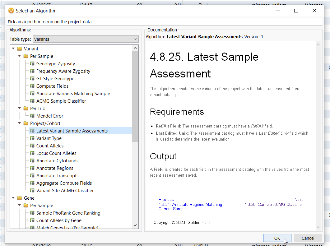
Recently, a Golden Helix customer reached out to support for advice on how to validate the variant scoring between two different VarSeq users. Here we break down one possible solution as an opportunity to showcase the utility of both the Latest Sample Assessment function and an alternative way to leverage the Compute Fields function. To set up this validation project, the Head Clinician first had his two evaluators take their validation sample and score variants using two separate Assessment Catalogs (for more information on how to use Assessment catalogs, check out these awesome blogs here and here). Once the two users had finished their separate assessments of their validation sample, it was time to compare their results and look for inconsistencies. To do this, let’s first go to Add > Compute Data where you can see an algorithm most people have not utilized. That is the Latest Sample Assessment algorithm (Figure 1).

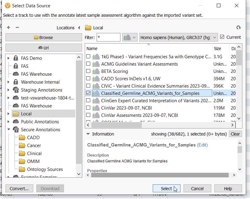
With this algorithm, you can select an assessment catalog that will annotate against your current project (Figure 2). This algorithm allows you to see the last time a variant was assessed, if ever, and the most recent classification. I did this process incrementally, first annotating my validation sample with the Classified Germline ACMG Variants catalog, and then again with a catalog called BETA Scoring.

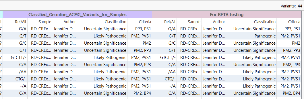
Now in my variant table, you can see that my variants have been annotated with several useful fields, including the name of the sample that housed the last classified variant, the author (yours truly for both these catalogs), and the overall Classification (Figure 3). Now if you were to stop here, you could theoretically ‘spot check’ for differences in the two Classification columns. For my 44 variant project, this could be feasible, but spot-checking differences is not practical if we move into a larger project with perhaps millions of variants.

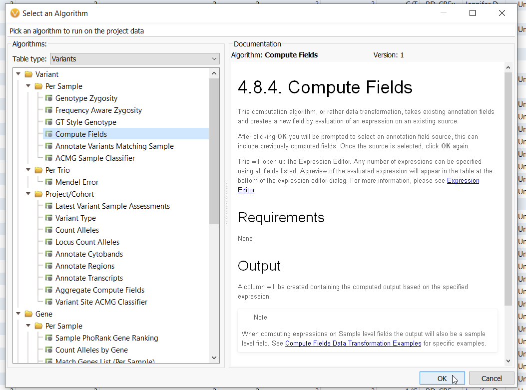
For larger projects, you are going to need a more automated solution, and this is where Compute Fields come into play (Figure 4).

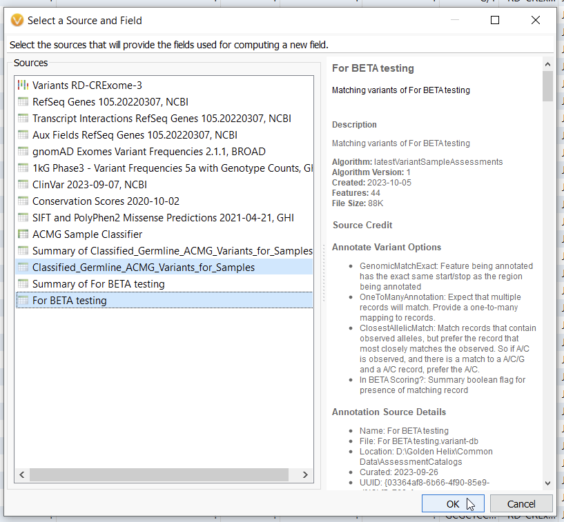
Most VarSeq users are not aware that they can bring multiple sources at once into the Compute Fields algorithm (Figure 5). Here I am bringing my two assessment catalogs, the Classified Germline ACMG Variants, and the For Beta testing catalog.

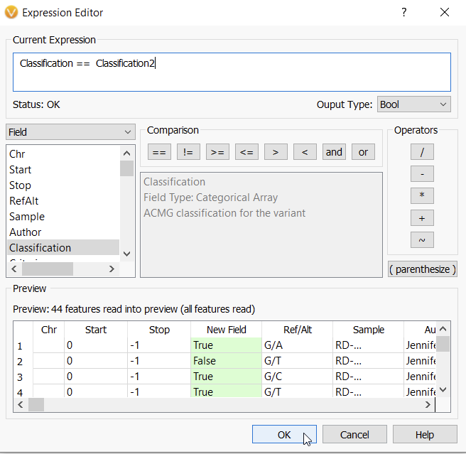
Next, I am going to define the parameters of my new function. Here I am taking the Classification field from the first assessment catalog, and comparing it to the Classification field (Classification 2) of the second assessment catalog (Figure 6). When done, I hit OK.

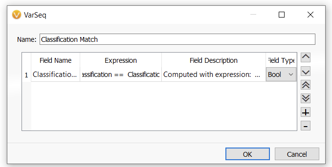
In this next window, I can give the new function a name (Figure 7). Here this will be a Boolean field (True vs False) with the name Classification Match. Then, hit OK.

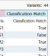
This has now generated a new column showing if the output from the two fields is in agreement (True), or in Disagreement (False) (Figure 8).

You can turn this column into a new filter where you can easily isolate and assess the differences in classification between the two columns (Figure 9). In this example, you can find where the two reviewers differently scored variants, making it easy to re-score if needed.

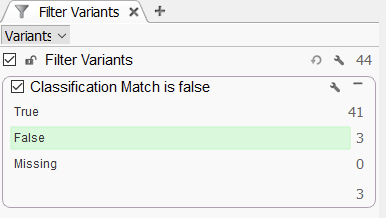
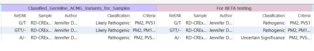
When clicking on the three ‘False’ variants, I can pull up the ones that were scored differently (Figure 10). In the first catalog, the G/T was Likely Pathogenic in the first catalog, while Pathogenic in the second. Next, we could take a look at the individual criteria to look for the differences, all while comparing the auto-Classification to the ACMG Classifier.

Overall, this was a quick look at how we can leverage both the Latest Sample Assessment algorithm and the Compute Fields Algorithm together to automate a quality control check. We hope that this inspires you to find other out-of-the-box uses for these very flexible algorithms. If you have any questions about how to make a compute function, please reach out to support@goldenhelix.com, and our FAS team would be happy to help you!