Last week Khanh-Nhat Tran-Viet, Manager/Research Analyst II at Duke University, presented the webcast: Insights: Identification of Candidate Variants using Exome Data in Ophthalmic Genetics. (That link has the recording if you are interested in viewing.) In it, Khanh-Nhat highlighted tools available in SVS that might be under used or were recently updated. These tools were used in his last three filtering steps to bring down the number of variants from 1,900 to only 9. However, there were three filtering steps used before he got to these last three steps that were not covered as part of the webcast.
In this post, I will walk you through all of the filtering steps and point out places where you can choose to either expand or contract the filters. To paraphrase Khanh-Nhat, when you consider which filtering steps to do in which order, you need to keep in mind what to do if your filters do not yield any interesting variants. In those instances, you would need to back up to the previous step and so, as you go along, consider your assumptions and how criteria might be loosened.
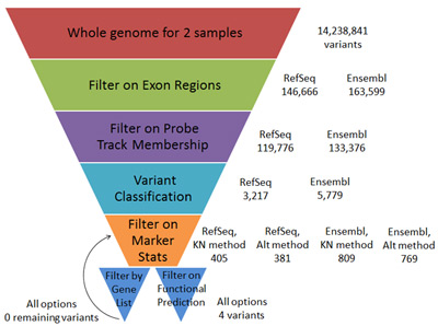 Note: You can use any of our DNA-Seq tutorial data to follow along with this blog post, but I will use a mother-daughter pair of whole genome samples from Complete Genomics from Pedigree 1463 (NA12878 and NA12885) to simulate the relationship between the two samples in Khanh-Nhat’s data. These samples can be downloaded from Complete Genomics, and while they are whole genome instead of exome only, the first step in Khanh-Nhat’s workflow will get us down to approximately whole exome size. To start, the two whole genome samples from CGI have 14,238,841 variants together. Please note that to follow along you will also need to download several annotation tracks, which are listed at the end of the post.
Filter by annotation track membership exon +/- 10 bp
From the webcast…
To remove the majority of intronic and intergenic variants, Khanh-Nhat began by filtering by annotation track membership exon +/- 10 bp in SNP & Variation Suite (SVS).
In SVS…
From a variant spreadsheet in SVS (you’ll need a “Reference” field in the marker map, contact [email protected] if you need help with this), go to Select > Filter by Annotation > Filter by Exon Region.
The default gene track selected is RefSeq Genes from UCSC. One of the last filtering steps used by Khanh-Nhat is filtering on dbNSFP NS Functional Predictions. The dbNSFP database was built off of EnsemblGene v63 exon regions. So if you leave the default gene track you could end up with variants classified as non-synonymous in one step that are not classified as non-synonymous in another. This could be desirable (or not) depending on if you want to limit yourself to only variants classified as Non-Synonymous by dbNSFP or not.

Results…
| Using RefSeq Genes (Default Track) | Using EnsemblGenes (Ensembl v63) |
| Filters down to 146,666 variants in exon +/- 10 bp regions | Filters down to 163,599 variants in exon +/- 10 bp regions |
Common dbSNP137
From the webcast…
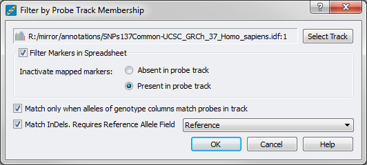
Khanh-Nhat used Common dbSNP137 to filter out variants that have a minor allele frequency greater than 1 percent. Alternatively, if you are looking for completely novel variants, you can filter on dbSNP137; however, this could remove too many interesting variants.
In SVS…
From a variant spreadsheet in SVS, go to Select > Filter by Annotation > Filter by Probe Track Membership and select the SNPs137 Common annotation track. Make sure to change the filtering behavior to remove variants present in the annotation track.
Results…
| Using RefSeq Genes (Default Track) | Using EnsemblGenes (Ensembl v63) |
| Filters down to 119,776 variants in exon +/- 10 bp regions with a MAF <= 1 % according to dbSNP137 | Filters down to 133,376 variants in exon +/- 10 bp regions with a MAF <= 1 % according to dbSNP137 |
Variant Classification
From the webcast…
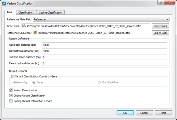
To remove the synonymous variants, Khanh-Nhat ran variant classification. Variant Classification uses the variants present in the data, a gene track to define coding exon regions, and a reference sequence track to obtain the reference alleles. Here again, the gene track can either be left as the default RefSeq Genes track or changed to the EnsemblGenes track.
In SVS…
To run variant classification, go to Analysis > Variant Classification.
Results…
| Using RefSeq Genes (Default Track) | Using EnsemblGenes (Ensembl v63) |
| Filters down to 3,217 variants in exon +/- 10 bp regions with a MAF <= 1 % according to dbSNP137, non-synonymous based on RefSeq Genes | Filters down to 5,779 variants in exon +/- 10 bp regions with a MAF <= 1 % according to dbSNP137, non-synonymous based on EnsemblGenes |
Filter by Marker Statistics
From the webcast…
Khanh-Nhat used Quality Assurance > Genotype > Genotype Statistics by Marker to choose the variants he was interested in. Instead of using this tool, he could have chosen to use Select > Activate Variants by Sample Genotypes or an add-on script Activate Variants by Genotype Count Threshold. I will show both Khanh_Nhat’s method and one alternate method.
In SVS (Khanh-Nhat’s Method)…
Khanh-Nhat’s goal was to filter down to variants that had a call for both samples and were also heterozygous for both samples. First, he went to Quality Assurance > Genotype > Genotype Statistics by Marker and selected all options except for the Hardy-Weinburg statistics (make sure to change the allele classification to be based off of Reference/Alternate).
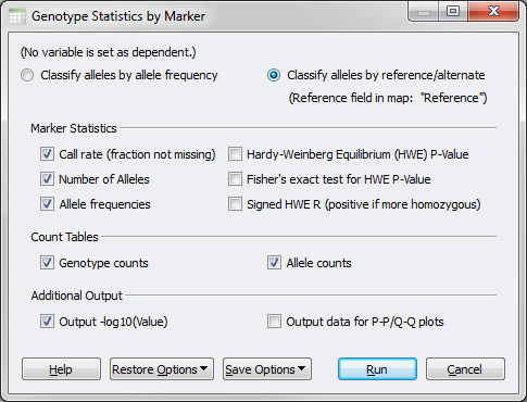
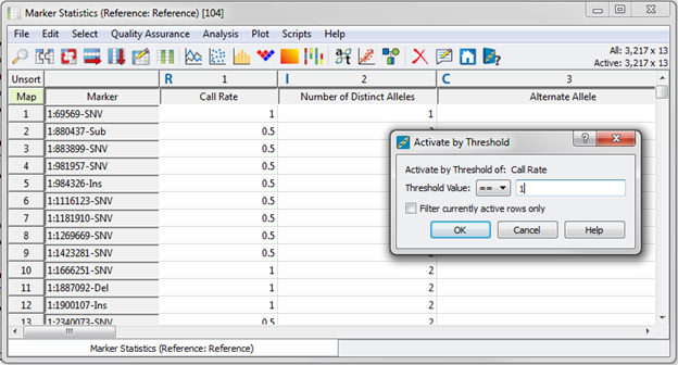
Next, click on the column header for Call Rate and select Activate by Threshold. Choose “==” for equals and enter in a value of 1 to get only those variants with a call for both samples.
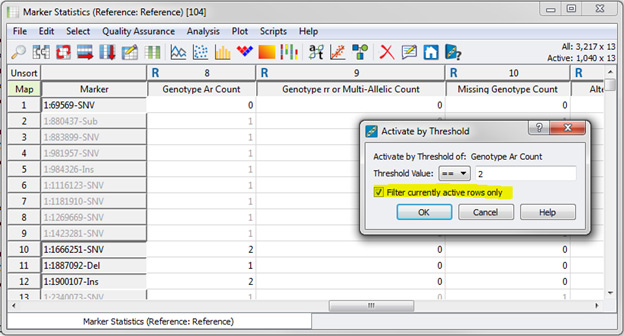
Then, click on the column header for Genotype Ar Count. Choose “==” and a value of 2. Make sure to check “Filter currently active rows only”. This filter will give us the variants where both samples have an Ar genotype which represents having one [A]lternate allele and one [r]eference allele, in other words heterozygous genotype calls.
To select only these variants in the genotype spreadsheet, Khanh-Nhat opened up the Genotype spreadsheet and went to Select > Activate or Inactivate based on Second Spreadsheet and chose the following options: “Set the state of Columns in the current spreadsheet to Active based on active… Rows in the specified spreadsheet” and selected the Marker Statistics (Reference: Reference) spreadsheet.
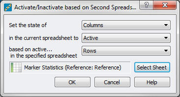
Note: Apply Filter to Spreadsheet can be used instead. With this tool start from the Marker Statistics (Reference: Reference) spreadsheet and go to Select > Apply Filter to Spreadsheet. Most of the time the prompts will have the correct selections detected automatically, but it doesn’t hurt to check that the filter will be applied to the correct spreadsheet, and that the correct dimension in the starting spreadsheet will be used for filtering.
In SVS (Alternate Method)…
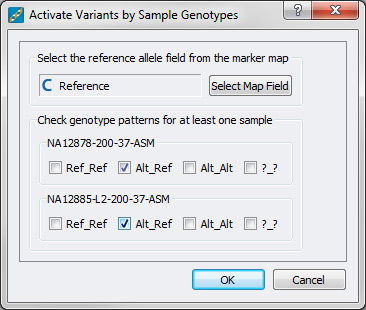
This could have been done in fewer steps by going to: Select > Activate Variants by Sample Genotypes and requiring that both samples have an Alt_Ref genotype. This will also filter out substitutions, Indels and where the genotype is heterozyous but both alleles are alternates.
Results…
| Using RefSeq Genes (Default Track) | Using EnsemblGenes (Ensembl v63) | ||||||||
|
|
Filter by Gene List
From the webcast…
The data that I am using obviously is not guaranteed to have any pathogenic variants in it, especially variants in ocular genes. But the purpose of this analysis is to work through a typical NGS workflow and adjust where required. So here goes! I grabbed a copy of the gene list from NEIBank and after some manipulation in Excel, imported it into SVS. All that is required for this is a column of Gene Names and some other identifier as row labels.
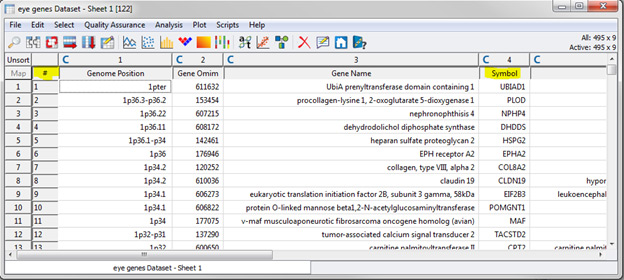
From the variant spreadsheet, go to Select > Filter by Gene List. Select the gene list spreadsheet and the column containing the HUGO gene name, or the name that will be used in the gene annotation track. In this case, it is the Symbol column.
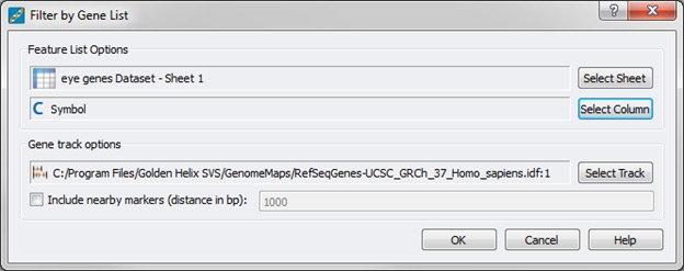
Results…
Unfortunately, none of the variants are found in this gene list.
| Using RefSeq Genes (Default Track) | Using EnsemblGenes (Ensembl v63) | ||||||||
|
|
What to do now????
Well, let’s back up. Our last goal was to find variants that were in the known ocular gene list. Since we didn’t find any, let’s just look in exon regions for all genes. Now, we’ll go back to the variants left after filtering on marker statistics (Call Rate = 1 and Ar count = 2) and continue on to the next filter.
Filter by dbNSFP NS Functional Predictions
From the webcast…
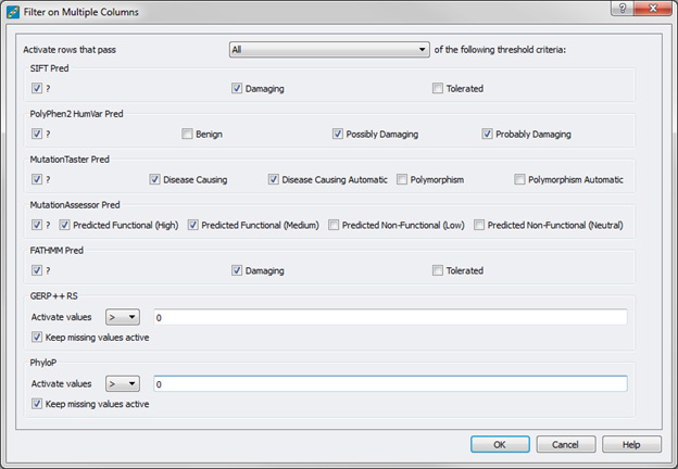
Khanh-Nhat required that his variants be classified as missing or damaging by the 5 functional prediction scores and as conserved by the two conservation scores in the dbNSFP NS Functional Predictions database. Let’s give this a try:
In SVS…
From the variant spreadsheet, go to Select > Filter by Annotation > Filter by dbNSFP NS Functional Predictions. If prompted, make sure you download the latest version of the dbNSFP annotation track if you have not already done so. The latest version is v2.0; v2.0b2 is “version 2 beta 2” while v2.0 is “version 2.0 final”. If you have SVS version 7.7.4, you will be prompted to get it if the latest version is not found. Make sure you select “Annotate only” instead of “Annotate and Filter”. Note, the other parameters do not matter since you are only annotating and not filtering.
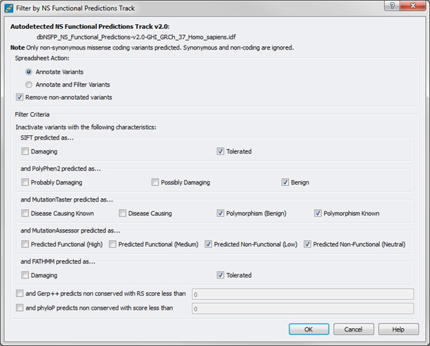
Once the report has been generated, go to Select > Filter on Multiple Columns. Select all of the “pred” columns and the two conservation scores (GERP ++ and PhyloP). In the following dialog, Khanh-Nhat required that the filter apply to all columns and he set the following options:
| Using RefSeq Genes (Default Track) | Using EnsemblGenes (Ensembl v63) | ||||||||
|
|
This is too many variants, now what???
Simple, let’s make a more stringent filter. Instead of including the missing predictions, let’s remove those too. Doing this now yields the same 4 variants no matter the method:
| Using RefSeq Genes (Default Track) | Using EnsemblGenes (Ensembl v63) | ||||||||||||||||||||||||
|
|
But what if my filter yielded no variants???
OK, so there are two options. Either you can back up another step and not require that the variants follow a dominant genetic model or you can loosen the dbNSFP filtering criteria. Before you drop the dominant model assumption, try easing the filtering requirements. So go back and Filter on Multiple Columns again. You can either specify the 7 columns again but this time say that “at least 6” of the criteria must be met or you can exclude one or more of the prediction algorithms and require that all of the criteria be met. Of course, if this still doesn’t work, you can go further back in the funnel and loosen the requirements there.
Now let’s take a peek in GenomeBrowse…
Let’s look at 12:103234252-SNV in GenomeBrowse™. GenomeBrowse allows you to visualize BAM files and investigate mutations quickly and easily. The data for these two samples came from Complete Genomics in Evidence files; I used cgatools to create SAM files and samtools to create BAM files.
Once the BAM files are created, they can be loaded into GenomeBrowse for visualization. In the image below you can see the BAM files for NA12878 and NA12885 as well as various other annotation tracks. Note that I am able to easily edit the labels to identify which sample is the daughter and which sample is the mother.
As you can see in the coverage and pile-up views for both samples, it is evident that this is a heterozygous mutation represented on both strands. Thus it is a valid mutation and not an artifact of a variant caller. The mutation is not seen in SNPs 137 Common (which is expected since we filtered those variants out) but is seen in the full SNPs 137 database. This again is expected since the samples we are examining are HapMap samples. The mutation occurs in the PAH gene and according to OMIM is associated with Phenylketonuria, 261600 (3); [Hyperphenylalaninemia, non-PKU mild], 261600 (3). This mutation was found in 4 European American samples in the NHLBI ESP 6500 Exome dataset. From here, I will leave the interpretation of this finding up to you!
Your Journey
I hope that you have enjoyed following along as we have explored the variant calls for these two samples. As a reminder, each filtering workflow is as unique as the data that you are filtering and your end goals. There are numerous filtering possibilities available in SVS, and I hope that you check out our other resources such as tutorials, blog posts, and webcasts to further explore how SVS can help you identify potentially causal mutations in your DNA sequence data.
If you would like to talk to someone about how to design a workflow for your situation, please email us at [email protected], and we would be more than happy to help you.
If you are already an avid SVS user, I hope that this journey has helped you discover new features in SVS or learn new ways to use the software!
—
Tracks required to follow along with this blog post:
RefSeqGenes-UCSC_GRCh_37_Homo_sapiens.idf
EnsemblGenes-UCSC_GRCh_37_Homo_sapiens.idf
SNPs137Common-UCSC_GRCh_37_Homo_sapiens.idf
ReferenceSequence-UCSC_GRCh_37_Homo_sapiens.idf
dbNSFP_NS_Functional_Predictions-v2.0-GHI_GRCh_37_Homo_sapiens.idf
