A few months ago, our CEO, Christophe Lambert, directed me toward an interesting commentary published in Nature Reviews Genetics by authors Bjarni J. Vilhjalmsson and Magnus Nordborg.  Population structure is frequently cited as a major source of confounding in GWAS, but the authors of the article suggest that the problems often blamed on population structure actually result from the environment and the genetic background of the study population.

Population structure (as often measured by principal components) serves as a proxy for both environment and genetic background, but does not entirely account for either one. The authors argue that the better approach is to estimate the relatedness of subjects based on their genotypes and include the resulting kinship matrix in a mixed model regression analysis.  They provide citations for several papers indicating that this approach outperforms common methods that adjust for population structure as a fixed effect.  It is a very concise and informative paper, and I encourage everybody involved in GWAS analysis to read it.

This article did not come as a major revelation to us at Golden Helix, as we had already been studying this approach for some time, with the particular encouragement of our clients in agrigenomics.  One of the major assumptions for a typical GWAS is that the subjects are unrelated individuals selected from a random mating population, and that assumption is almost impossible to satisfy in modern agriculture.  As a result, the plant and animal genetics community has been very active in developing statistical techniques to compensate for extensive relatedness and population structure in GWAS. For example, TASSEL, a software tool broadly used in agrigenomics research, has incorporated a mixed model framework to account for population and family structure since it was first described in 2007.

Mixed model analysis is quite common in non-human GWAS applications and is being used in human research with increasing frequency.  I am pleased to inform our readers that mixed linear model (MLM) regression analysis will soon be available in SVS, providing the capability to adjust for genetic background by including IBS kinship estimates as a random effect in GWAS analysis.  There is a working prototype in testing right now, and the functionality will be available to SVS users in the next few weeks.

MLM Case Study
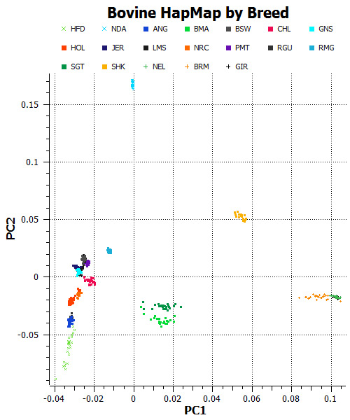
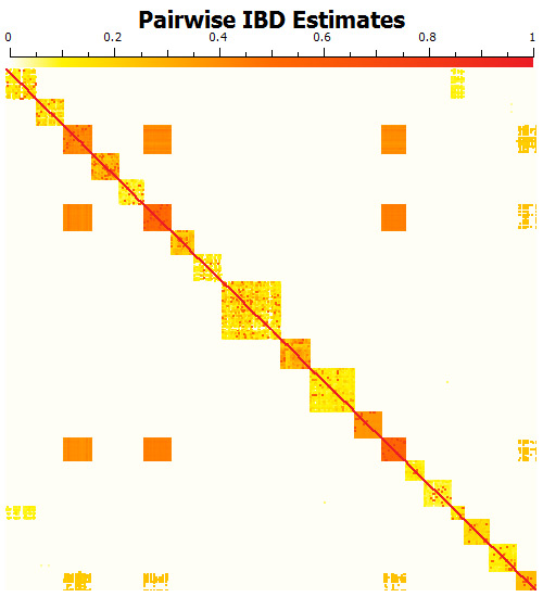
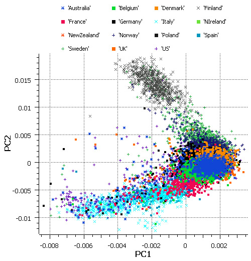
As a case study for the current MLM prototype, I analyzed data from the Bovine HapMap project with 472 cattle representing 19 different breeds that were genotyped with Illumina’s 50k bovine chip.  The plots below give an idea about the degree of population structure present in the data.

Figure 1: Scatterplot of the first two principal components of the Bovine HapMap data, stratified by breed. Most animals are from species Bos Taurus, but the three breeds at the far right (NEL, BRM, and GIR) are from species Bos Indicus.

Figure 2: Heatmap of pairwise IBD estimates for the 472 cattle in the Bovine HapMap data. The blocks along the diagonal are breed groups. Within breed groups, it is common for pairs of “unrelated” animals to have IBD sharing estimates between 10% and 40%, as each breed has varying degrees of homogeneity. The blocks away from the diagonal indicate that some pairs of breeds are genetically similar to one another.

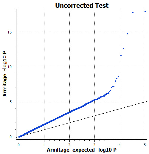
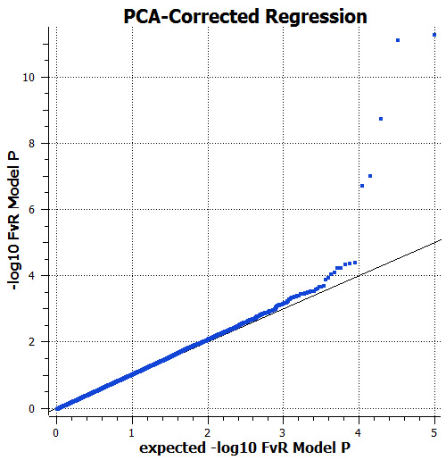
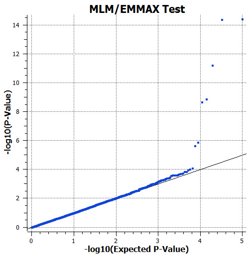
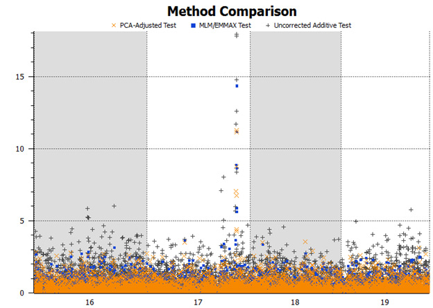
I simulated a binary phenotype with a few breeds being over-represented in the case group.  The phenotype was simulated to have a strong association on bovine chromosome 17.  I filtered the SNPs to have call rate > 0.95 and MAF > 0.01 and proceeded to run three association tests: 1) an additive association test with no adjustments; 2) a logistic regression using an additive model and adjusting for population structure using principal components; and 3) an MLM association test adjusting for genetic background in an EMMAX framework.  The first two tests were done using standard methods available in SVS, while the third test utilized the current SVS MLM prototype.

All three tests correctly identify the simulated disease locus, but the P-value distribution across the remainder of the genome is very different.  The uncorrected test shows uniform inflation of significance.  The PCA correction and MLM approaches both effectively reduce the inflation of P-values, but the significance assigned to unassociated loci varies somewhat between the methods.  Which approach is correct?  You be the judge.

Figure 3: Observed and expected P-values for the unadjusted additive association test. There is uniform inflation of significance throughout the genome (lambda = 2.42), apparently because the phenotype is correlated with breed, and breed is correlated with markers throughout the genome.

Figure 4: Observed and expected P-values for the logistic regression test correcting for population structure by including principal components as a fixed effect. The inflation of significance from the unadjusted test is effectively removed by this approach. Several SNPs remain significant.

Figure 5: Observed and expected P-values from the MLM test correcting for genetic background by including the IBS kinship matrix in the analysis model. The inflation of significance from the unadjusted test is effectively removed by this approach. Several SNPs remain significant.

Figure 6: Comparison of the P-values generated by the MLM test and the PCA-corrected test. The two methods agree on the most significant results, although the MLM test assigns greater significance to those SNPs.

Figure 7: Detail view of the Manhattan plot showing results of the three tests; -log10 P-values are shown for chromosomes 16 through 19. The increased background significance of the uncorrected tests is clearly evident.

Not Just for Animals
During the latter part of 2012, I was involved with an analysis project that incorporated data from the WTCCC2 Multiple Sclerosis (MS) GWAS.  There are some very unique challenges associated with that dataset.  The data includes more than 11,000 MS cases from all over Europe, North America, Australia, and New Zealand together with an even larger set of controls.  While cases were collected in 15 countries, over 60% of the controls came from just two countries (USA and UK).  There were substantial numbers of cases from several countries — including Spain, Australia, New Zealand, Belgium, Poland, and Ireland — for whom there were no geographically matched controls.  The large sample size works together with the population structure to create a data resource with high potential for confounding in GWAS results.

Figure 8: The first two principal components of the WTCCC2 MS cases, stratified by country of origin.

The original WTCCC2 MS publication in Nature describes the analytic odyssey that the researchers experienced as they worked to get the best possible GWAS results (as usual, the best parts of the story are in the supplementary material).  A standard frequentist analysis of the data showed substantial inflation of significance, with lambda=2.48 even when the MHC region (which is overwhelmingly associated with MS) was removed.  They proceeded to adjust the test for principal components and determined that there were seven components capturing genome-wide structure.  After adjusting the analysis for those seven components, lambda was still 1.21, which is unacceptably high.  They proceeded to use an MCMC clustering algorithm to identify ancestry-matched subgroups of cases and controls, performed association tests within subgroups, and combined the results in a meta-analysis.  The inflation factor in the result was even worse than the PCA correction method, with lambda=1.44.

I’ll quote from the text of the supplementary material what they did next:

“Our third approach was to use a linear mixed model that explicitly accounts for correlations in individuals’ phenotypes due to their relatedness. One major advantage of this approach is that it accounts for structure due to relatedness on multiple time scales, from close relatives to distant ancestral structure. We generated a covariance matrix R by calculating for every pair of individuals the genome-wide averaged correlation among their genotypes. This corresponds to a method of moments estimate of the proportion of genome related identical-by-descent between two individuals sampled from the population. Linear mixed models that incorporate this type of measure of relatedness in a GWAS setting have been used before. In this study we use a novel implementation described below…”

To paraphrase, they took the same basic path suggested by Vilhjalmsson and Nordborg, using a mixed model approach that explicitly accounts for the observed relatedness of each pair of subjects.  It is important to note the language they use — that the model accounts for phenotypic correlations.  This seems counter-intuitive at first, given that the correction factor is calculated not from phenotypes but from genotypes.  But Vilhjalmsson and Nordborg explain this concept in their article:

“In a groundbreaking 1918 paper, Fisher showed how the phenotypic covariance between relatives depends on their genetic relatedness, assuming that phenotypic variation was due to the additive effects of a large number of loci of small effect. The basic idea is very simple: the more alleles that individuals share, the more similar they will be. In human genetics, the same logic underlies the Haseman–Elston regression, and in animal breeding the classic Henderson mixed model has been used to reduce the confounding effects of genetic background when mapping in pedigrees.”

It’s funny how everything in statistics always leads back to Fisher.  Phenotypes are the outward expression of genotypes, so by accounting for genotypic similarity, we are also accounting for phenotypic correlation, and hence the reason that the WTCCC2 report uses that language.

The application of the mixed model approach for the WTCCC2 MS project was very successful.  The lambda statistic was reduced to just 1.04 with this method, well within acceptable limits.  Given that this analysis also had issues with genotyping platform effects (the cases were all genotyped with a customized Illumina 660 chip, while the controls used a variety of different Illumina platforms, and our analysis showed clear evidence of the effects of that, but it is a topic for another day), this result is an excellent outcome for a very challenging analysis.

The MLM approach isn’t appropriate for every analysis.  Vilhjalmsson and Nordborg mention a few of the limitations, and point out examples where the best analysis models included both relatedness and direct estimates of population structure.  I am still learning the benefits and limitations of the method myself, and am excited by the prospect of a new tool to use in my analysis work.  The MLM methodology will be available soon in SVS, and we look forward to getting more feedback from users about how we can continue to make SVS even more powerful and useful.