If you’ve seen the recent webinars given by Gabe Rudy and Bryce Christensen, you’ve no doubt been impressed by the capabilities of VarSeq when it comes to annotation and filtering. However, we sometimes forget that the power that enables all this complex analysis can also be used in more mundane tasks like VCF subsetting. And although these day-to-day tasks don’t make for an impressive demo, they are central to the work of anyone who deals with genetic data.

Some might scoff at the idea of using a full featured application for basic bioinformatic tasks, when excellent open source tools can get the job done. I completely agree and am the first to defend, support, and contribute back to the open source community.

However, open source tools are often command line focused, which means that the user needs to be comfortable at a command prompt and have a decent shell available (which isn’t always the case). The barrier to entry for using these programs is actually much higher than simply having command line access. Usually you’ll need to know about “cloning a repo”, “having all the dependencies”, and “running make”. Even as a developer who spends 50% of my day at my shell prompt, I am sometimes frustrated with how long it will take me to do a “simple” task that requires a tool I don’t already have.

VarSeq and the command line square off on my desktop

In this light, I decided to do a side by side comparison of a basic bioinformatics task using both VarSeq and the command line.

Often, we are given a VCF file that contains many low quality variants. These low quality variants bloat the data and it becomes difficult to work with — each analysis step takes an order of magnitude longer, file transfers become a hassle, and generally analysis is less productive.

A common solution in whole exome trio analysis is to remove variant sites where the proband’s sequence quality is clearly too low to make an informed decision. Filtering only on the proband’s quality still allows you to use marginal parental calls as supporting factors in your analysis.

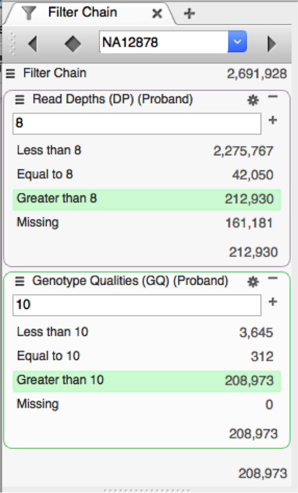
In this comparison, we’ll remove all variant sites where the proband’s genotype quality is less than 10 and where there are fewer than 8 reads supporting the call for the proband. This is a very coarse filter and you’ll probably still want to do additional filtering later.

There are a variety of command line tools to do this type of work, but my favorite is bcftools. Since it is made by Heng Lei’s team and backed by htslib, you know it is blazingly fast, accurate, and stable.

To fairly compare the two programs, I set out a few ground rules.

1. Both tools would be preinstalled. This actually removes a big technical hurdle from using bcftools. If it wasn’t pre-installed, you’d need to download the source code and compile it from scratch. Depending on your platform this could be difficult or impossible (I’m looking at you, Windows). However, if you are doing a lot of bioinformatics you’d likely have a linux box with the tools pre-installed.
2. I’d do a dry run with bcftools and record my commands so that I wasn’t fumbling with what flags to pass. Then I would just retype the commands. Since I hadn’t used bcftools in a while It actually took me 15 or 20 minutes to figure out the exact commands, but I assume for a bioinformatics analyst familiar with the tool it’d be second nature.
3. Both tools would get the same input and be required to produce the same output — a VCF file.

The results (drumroll):

• bcftools: 5 minutes 46 seconds
• VarSeq: 3 minutes 58 seconds

So what was the bottleneck on each tool? For bcftools, it’s my typing speed. Just typing commands was probably 50% of the time for bcftools. For VarSeq, it’s importing the VCF file. Importing this trio of more than 2 million variants took close to 2 minutes.

The filter chain in VarSeq makes it easy to see exactly what filters you are applying and what effect they have

It’s worth examining what these bottlenecks imply. In the case of bcftools, it just shows that I didn’t spend enough time with Mavis Beacon as a kid. However, those 2 minutes in VarSeq are actually time well spent.

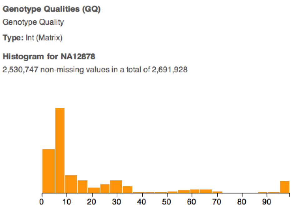
During import, VarSeq pulls your data into a read optimized database. This allows the program to do extremely fast real time filtering. This pays dividends when you decide that actually a read depth cutoff of 10 is more appropriate. Instead of another 5 minutes of command line tinkering, it’s literally 5 seconds. Moreover, VarSeq allows you to intelligently pick these cutoffs using a visual representation of your dataset. And as Anscombe’s Quartet proves, it always pays to visualize your data.

With the built in visualization of your imported data, you don’t have to guess where to set cutoffs

VarSeq additionally allows less technically skilled users to prototype their own annotation and filtering pipeline. Then if an analysis pipeline is already in place, they can tell their bioinformatics core exactly how they’d like their data to be run. The bioinformatics core engineer then has a perfect spec to develop a pipeline and even has test input and output files to benchmark the new pipeline against.

Command line tools will always be useful in analysis pipelines to automate tasks that are done the same way every run. But, for the one-off, day-to-day analysis and data wrangling that makes up a large portion of our day, VarSeq can make a dramatic difference in productivity.