Bioinformatic freedom is core to the user experience with Golden Helix software, a topic with which you will be well-versed if you’ve kept up on our recent blogs. We are constantly endeavoring to provide our users with powerful tools to tackle complex and impactful next-generation sequencing (NGS) workflows while maintaining transparency and the ability to customize and augment each component of a given pipeline. We’ve recently expounded quite a bit on our high-level automation tools and the wealth of prioritized information VarSeq curates via algorithms like VS-PGx and evaluation scripts in VSClinical ACMG and AMP. However, today, I’d like to go back to the basics and explore a fundamental and powerful tool within the foundations of any VarSeq workflow: Compute Fields.
Creating Custom Fields for Deeper Insight
VarSeq is unique in the NGS tertiary analysis space in that we allow users the full scope of information from their secondary analysis pipelines. Compute Fields allow users to go one step further. While VarSeq comes with a multitude of useful algorithms for a wide scope of applications, sometimes users require some specific, trenchant field to streamline analysis. This is where Compute Fields come in.
Compute Fields allows users to take arbitrary fields from a VarSeq project, from read depth to pathogenicity score, and combine them in unique, open-ended ways. So think up your most niche dream field, and let’s explore how we can access Computed Fields to bring it to life.
Navigating Compute Fields Step by Step
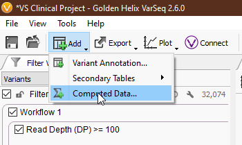
Compute Fields can be a little overwhelming at first, so let’s break things down step by step. To access Compute Fields, navigate to ‘Add > Computed Data… > Variant > Per Sample > Compute Fields’ (Fig 1-2).
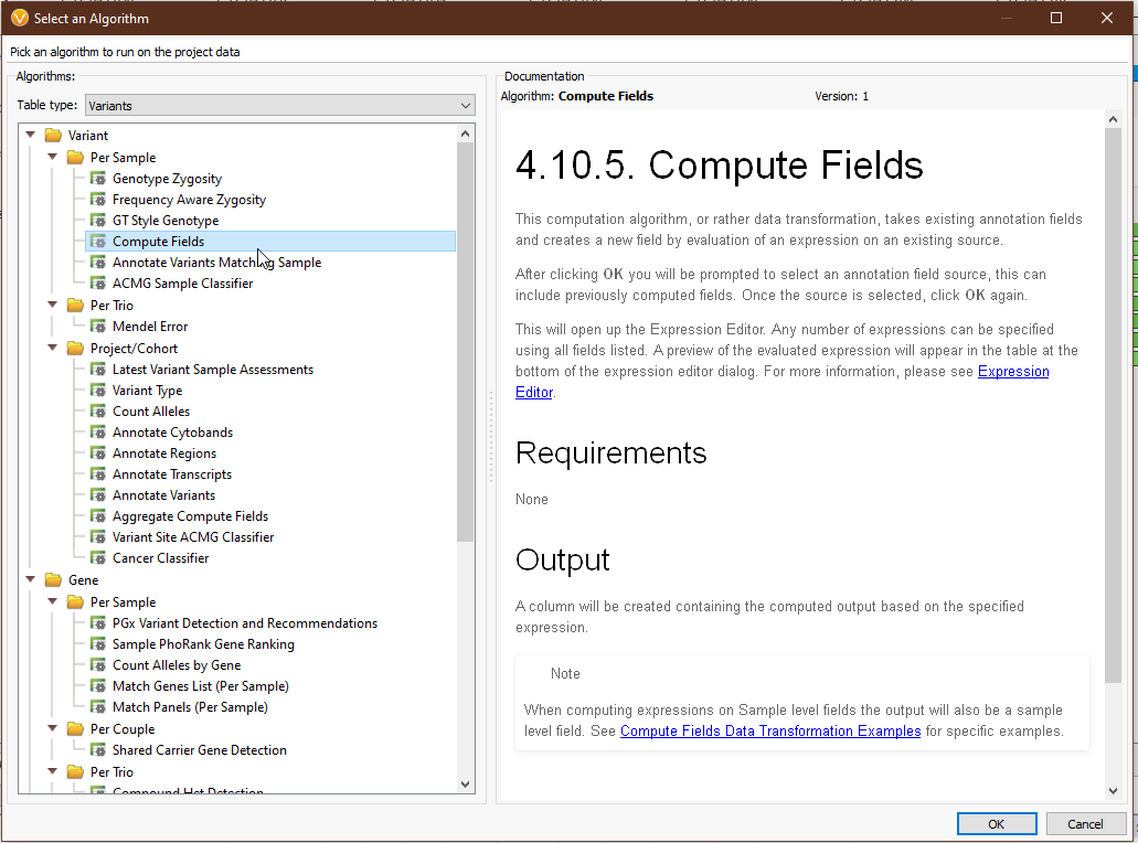
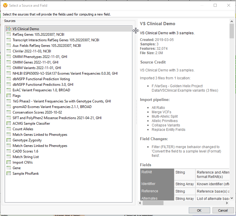
Clicking ‘OK’ will present us with a list of annotations whose fields we can use in Compute Fields. You can select a single annotation or multiple with ‘ctrl’ and ‘shift’ (Fig 3). For our example, we’ll stick with the first option, the variant format fields directly from our VCF. This will bring up the Expression Editor. This is where the magic happens. Let’s go through the important components.
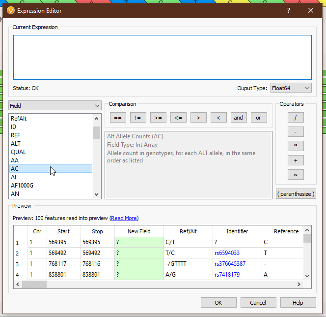
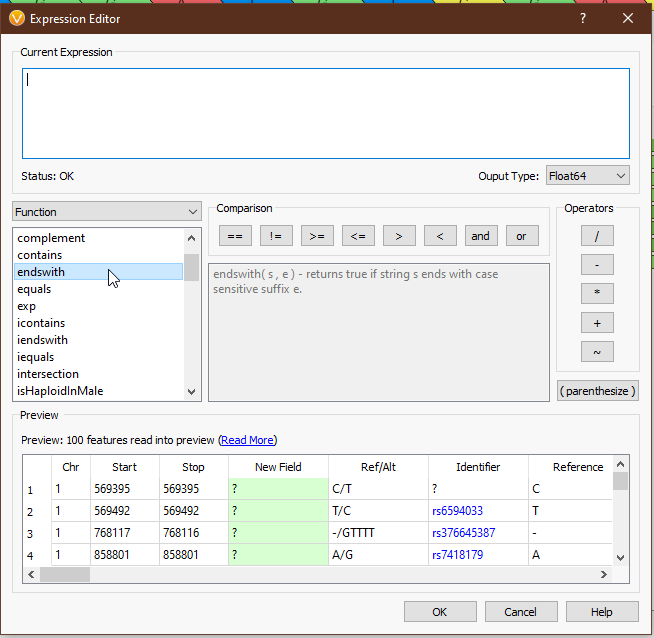
From the drop-down menu on the left, we can access all of the tools we have available (Fig 4). ‘Field’ provides the list of available fields from the previous selection. In this case we see things like ‘Chr’, ‘Start’, ‘Stop’, ‘AC’ (allele count), and other fields directly from our VCF. ‘Functions’ comprises all of the available functions that take field input(s). ‘Binary Operator’ contains all of the binary operators, such as comparison and arithmetic operators. ‘Prefix Operator’ and ‘Postfix Operator’ are unary operators that probably spark joy in the nerdiest of bioinformaticians and will be largely useless to anyone else. Lastly, ‘Constant’ contains e and pi (who knows when you’ll need to calculate the area of a circle whose radius is the read depth of a variant?). Single-clicking on any value will display the documentation for that field or operator (Figs 5-6), and double-clicking will populate that value in the ‘Current Expression’ section.
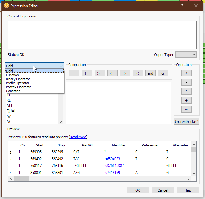
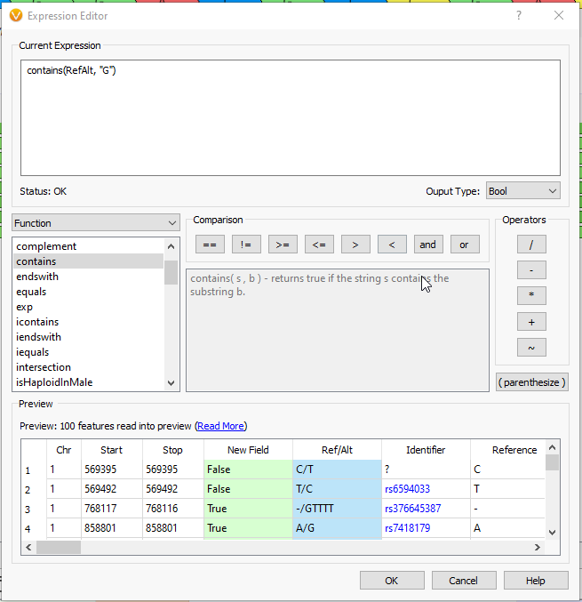
As an example, suppose we want to calculate a boolean field to determine whether there is guanine in the reference or alternate. We can use the ‘Ref/Alt’ field and the ‘contains function’; a preview of the results of the expression is displayed in the ‘Preview’ section (Fig 7).
From here, we need only select okay, give our new field a name, and then apply it to our heart’s content in our workflow. While this is a simple example, hopefully, it illustrates the ease of use with Compute Fields and gets the more ambitious bioinformaticians out there scheming how best to wield this tool.
As always, don’t hesitate to contact [email protected] with any specific questions. We look forward to seeing how you improve your workflow with Compute Fields!