SVS is a project-oriented program that manages and analyzes genomic datasets. This webcast statistically and visually explores the relationships among genetic variants within a cattle dataset. Even further, this webcast evaluates genotypes with corresponding phenotypes to assess how well a model can predict a phenotype of interest.

Starting with genotypic data from the microarray and the recorded phenotypic data for each sample, we are ready to perform an association test on our raw genotypic data. From the association test, we want to look for inflation in our markers significance and then look at where the significant regions are in the genome.  

Manhattan plots can be easily generated and customized to show where each SNP is within the genome and can be color-coded by chromosome to easily identify regions that may stand out for significance (Figure 1).

We want to be sure that the SNPs displayed in our Manhattan plot are not over-inflated. A correlation/trend test can be performed with ease in SVS and can quickly generate a Q-Q plot which will show expected vs observed -log10 P values and point out any inflation in the data. This will help illuminate the need for quality control of the sample, markers, and underlying sample relationships. (Figure 2).

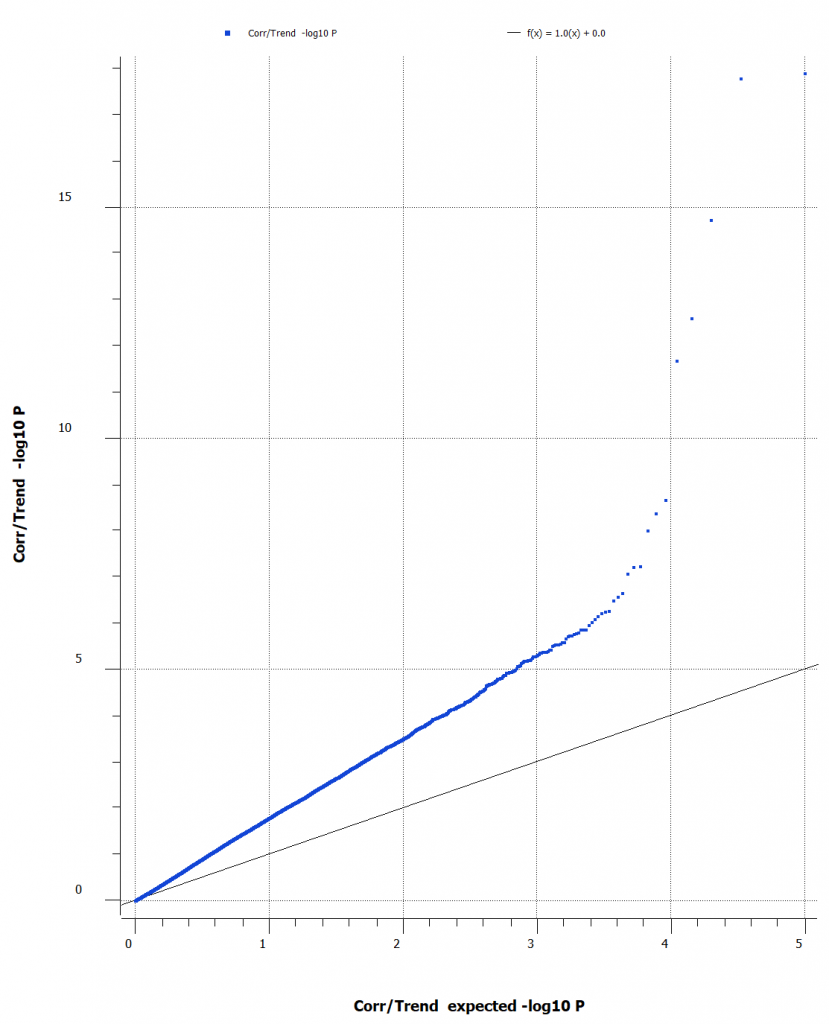
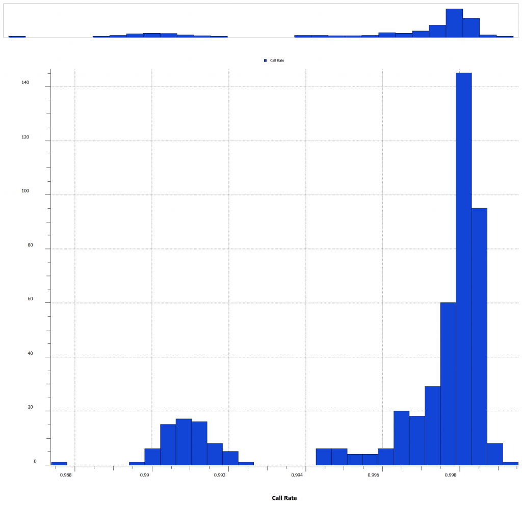
The Q-Q plot indicates that the data may have inconsistencies that should be considered and SNPs that should be filtered out. There are several features that SVS offers to edit, manipulate, and enrich your data. For most workflows, it can be helpful to calculate sample statistics to acquire information about the samples in your project. It is important to note any outliers, samples of poor quality, or possible sample duplications. A great metric that can be leveraged in this case, is the sample call rate. Figure 3 (below) is a histogram of the call rates of SNPs within each sample. To exclude samples that have too low of call rate and the user can determine what threshold to use.

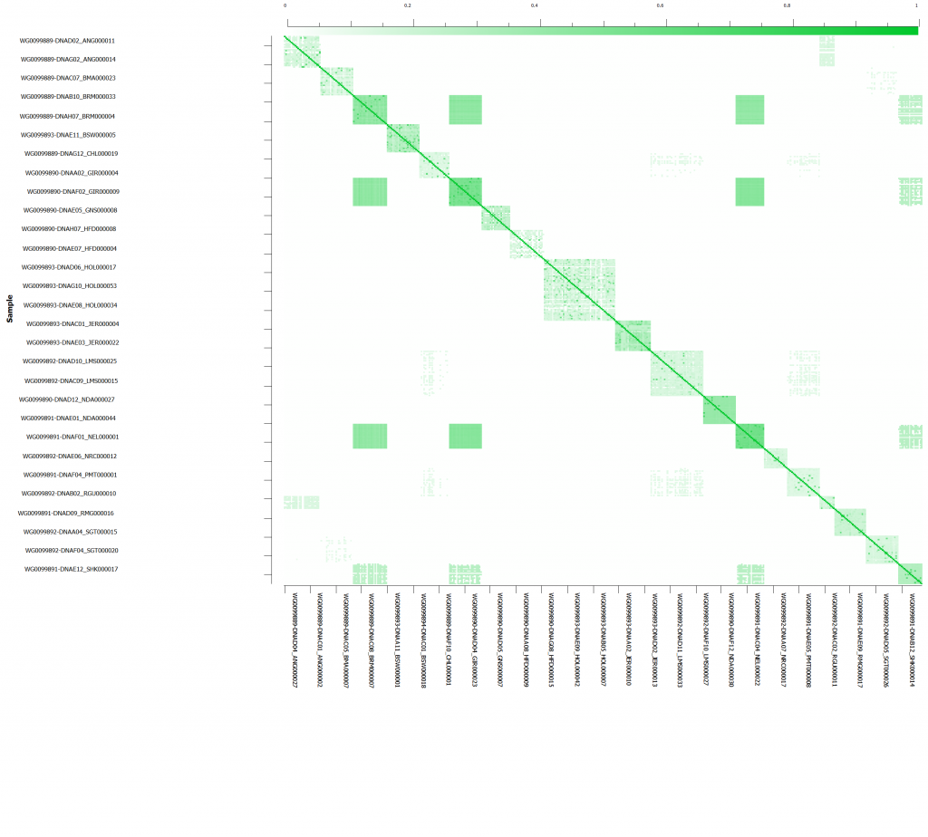
After sub-setting down to the call rate filtered SNPs, we will want to check to see which samples are related to eliminate the over representation of similar genotypes/haplotypes. Prior to sample relatedness, we want to eliminate any markers in linkage disequilibrium. Following LD pruning, sample relatedness can be assessed via IBD/IBS estimation. We can perform IBD to understand the proportion of alleles that appear to be from common ancestry. In addition, IBD pairwise estimates can detect duplicate samples and sample contamination ensuring further quality control (Figure 4). Then underlying population structure can be considered using Principle Component Analysis (PCA).

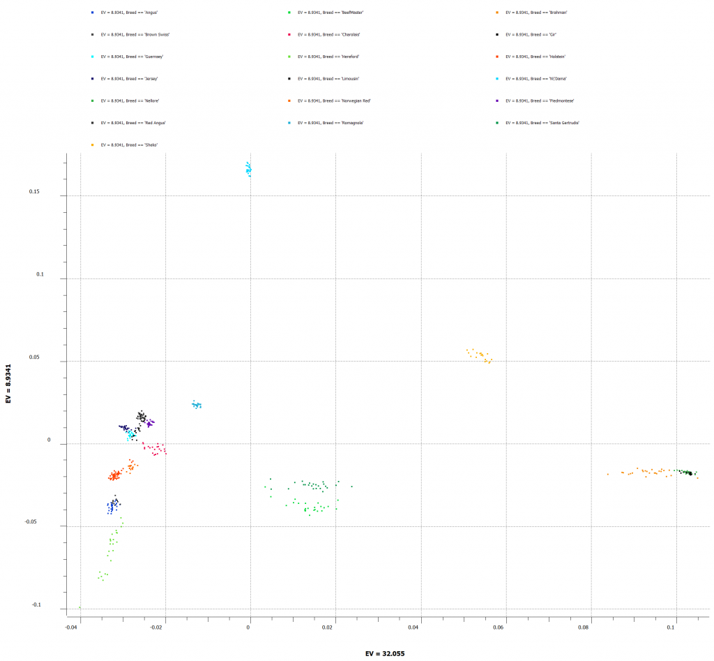
PCA will correct for any underlying population stratification amongst the samples. This can be done by comparing the top 2 principal components against reference samples of known breeds. Figure 5 shows all of the cattle breeds in our project and which breeds may be more closely related.

At this point, the association test can be re-run for the dataset wherein quality control metrics were applied. Now, we are ready to use genomic prediction with K-Fold to determine how well we can predict our desired phenotype from the known genotypic and phenotypic information from our cattle dataset.

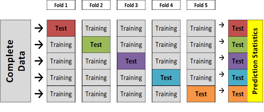
When setting up the genomic prediction, the K-Fold cross validation method is desirable because we want to estimate how accurately our predictive model (gBLUP or Bays C-pi) will perform on our dataset. By creating K number of subsamples using the stratified random sampling method, we can use all of our data for both training and testing.  Figure 6 illustrates that in each fold, a different sample’s phenotype set to missing and the remainder of the samples in the subset will predict the phenotype for the missing phenotype.

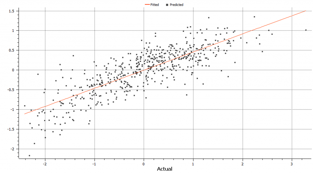
We can use the K-Fold cross validation and perform both Bays C-pi and gBLUP genomic prediction methods. The gBLUP linear based model where the algorithm uses a genomic relationship to encode covariance between samples based on observed genotypic similarity instead of ancestry and variance remains constant throughout calculation (Figure 7).

On the other hand, Bays C-pi genomic prediction algorithms use prior possibilities and quality beliefs about the data as well as conditional probabilities for a parameter based on the data (Figure 8).

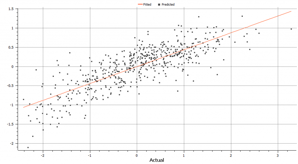
In this case, the models performed similarly, and gBLUP runs much faster. However, Bays C-pi may be preferred over gBLUP in the case when significant QTL exist.