2017 was a busy year regarding the development of our CNV tools. Since the release of the CNV caller, we have produced quite a bit of content tailored to assist our users with getting started.
Here are some links:
- Robarts Research Institute CNV analysis on patients with familial hypercholesterolemia
- CNV annotations
- Common CNV questions
- CNV calling with shallow whole genome sequencing data
In some cases, our users have approached testing our CNV caller against a set of validated events to see how our tools stack up. This process can be incredibly rewarding given that our tools are fully capable of detecting the calls you already know are there. However, what about confidence in calls that are unknown; how can you best utilize the software to assess these calls? The focus of this blog series is to first touch on the basics of building a CNV project, and next explore some specific features of the CNV calling process to prioritize events with the strongest evidence.
First off, let’s go over the basics.
Step 1: Collecting your data.
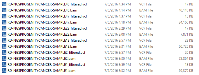
There are some important considerations when thinking about the sample data you are using to detect CNVs. The basis of calling CNVs in VarSeq is on coverage data stored in the BAM files. So, when collecting your data for import, be sure to have the BAM files for each sample VCF you are going to import into your VarSeq project (Fig 1).
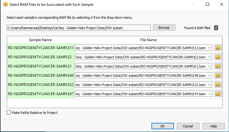
To import your BAM files, you’ll start the import process in VarSeq by selecting the VCF files and eventually reach the window seen in Fig 2. From here select the Associate BAM File icon. The next window will show you the paths of the BAM files that match each VCF. VarSeq will help you with this step by automatically linking the BAMs to their VCFs based on matching sample names. However, if things don’t match up, the user can always browse to the files manually (Fig 3).

Step 2. CNV prep: Building the reference set
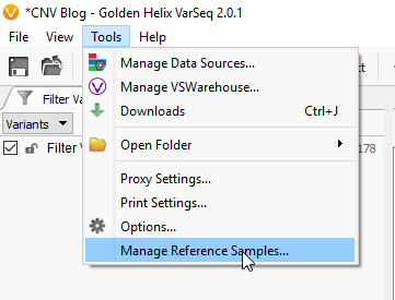
For the sake of simplicity let’s title our six imported samples as the samples of interest (SOIs). These are the samples we’re going to be searching for CNVs in VarSeq. I mentioned earlier that our CNV detection is based on coverage data in the BAM file for each sample. Any CNV present in any sample will be seen as a change in coverage over a specific region. To detect these changes in coverage, we use reference samples to create a sense of “normal” coverage and compare it to the coverage in our SOIs. Before we can detect the events, or change in coverage, in our SOIs we need to build our reference sample set. To do this, click Tools -> Manage Reference Samples (Fig 4).
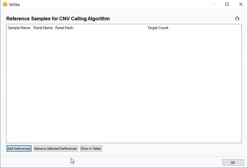
The window that pops up will be empty if this is your first time building a reference set. Click the icon to Add References to build your new reference set (Fig 5). The next window will look similar to the basic VarSeq importer, except you’ll notice now we’re importing BAM files, not VCFs (Fig 6). Since the CNV detection is based primarily on coverage data, we’re only utilizing the BAM files for our reference samples.
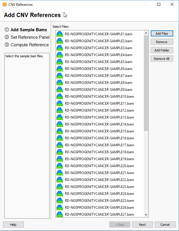
The next window is worth providing some additional explanation. There are two approaches to calling CNVs in VarSeq (Fig 7).
Approach 1: Target References for the Target Region coverage
- Use case – most suitable for gene panel/exon data with at least 100X or greater coverage.
- Coverage normalization occurs over regions defined by a bed file/interval track.
Approach 2: Binned References for Binned Region coverage
- Use case – most suitable for shallow whole genome sequencing data >100X down to less than 1X coverage!
- Coverage normalization occurs in binned regions over the entire genome (user sets bin size with the minimum being 10,000 base pairs).
This is an important step when building your reference set. You want to match the reference samples to your SOI’s by choosing the same options when preparing to run the coverage statistics (next step). For example, if you import a WGS sample into VarSeq with an average of 30X coverage, you’ll want to use the Binned Reference option for your WGS reference set.
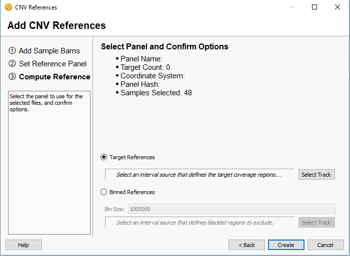
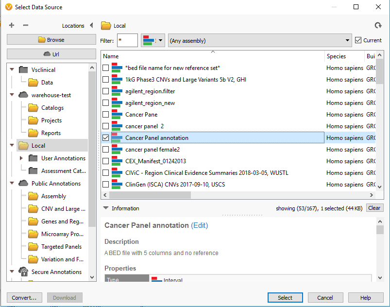
For this project, I am looking at gene panel data. So, I will define my reference set with the Target Reference option using an interval track/bed file defining my regions (Fig 8). It is common for our users to already have the bed files defining these regions, and if so you can import it into the software to create a region based annotation file to add to our list of curated databases. If you need any assistance with this step, please do not hesitate to email [email protected] so we can set up the bed file/interval track properly. Once integrated, the interval track can then be selected for the target regions (Fig 9) and final step is to click create.
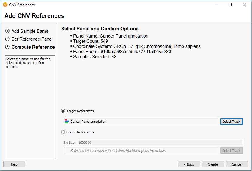
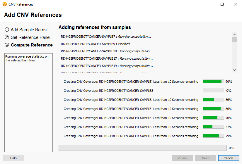
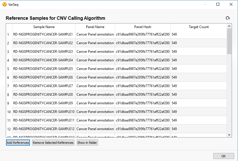
Now you will see the coverage statistic calculate for each of the reference sample you selected (Fig 10). Once completed, the newly added references will appear in the initial Manage Reference Samples window (Fig 11).
Step 3. Computing Coverage Statistics for our imported samples (SOIs)
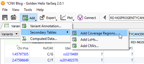
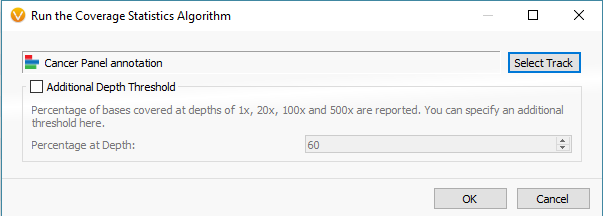
The last phase of the previous step was to run coverage statistics on the reference samples. We are going to achieve the same goal now with the imported samples of interest (the six imported SOIs). Following the targeted region approach, you can access the Compute Coverage Statistics algorithm by clicking Add -> Secondary Tables -> Add Coverage Regions (Fig 12 a). The next menu will be where you select the desired interval track defining the targeted regions. This important step is where you link the SOIs to the specific interval track defining target regions, which also selects the associated reference samples that match the interval track (Fig 12 b).
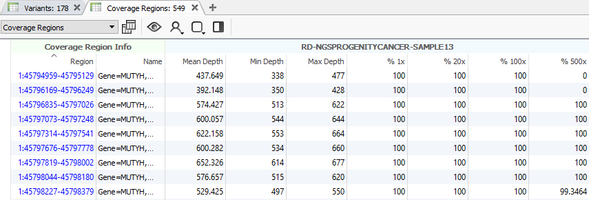
After running the coverage statistics algorithm, a new table appears listing the coverage information for each region defined by the interval track (Fig 13). The next step will be to compute CNVs, but there are some additional points to discuss beforehand.
Additional point 1: Coverage statistics on binned regions
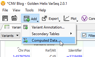
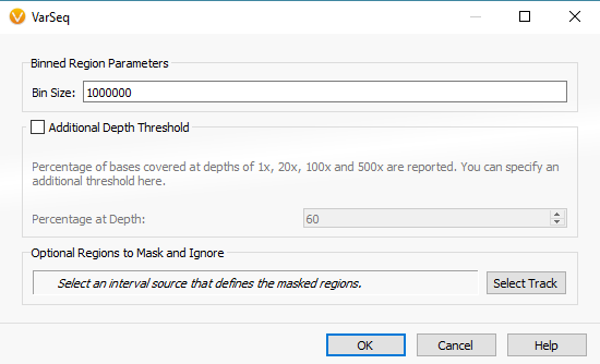
The example workflow in this blog follows the targeted region approach. However, if you are running the binned region approach for your whole genome data you will click on Add -> Computed Data (Fig 14 a). From the list of algorithms, select to run the Binned Region Coverage (Fig 14 b). When setting up the algorithm, the user will set the bin sizes across the genome (Fig 14 c) This is similar to the targeted regions in that the reference samples bin size needs to match the SOI bin size. So, if your reference samples were set to a bin size of 10,000 bp, you would also select 10 kbp when computing coverage for the SOIs.

Additional option 2: Running Loss of Heterozygosity
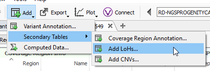
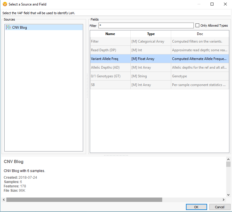
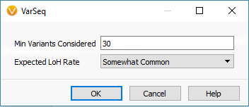
Another feature that you can add to your CNV analysis is the Loss of Heterozygosity (LOH) algorithm. This algorithm can be found in the quick access Secondary Tables options also (Fig 15 a). The LOH algorithm is a great way to help validate CNV calls and is based on variant allele frequency coming from the VCF file rather than the coverage data (Fig 15 b). Think of it as a secondary metric that adds another layer of evidence to reinforce CNV events you are validating. In this example project, the LOH caller is not run due to having a small gene panel with so few variants. This is an important recommendation that our users should know. As you prepare to call CNVs, VarSeq will prompt you with an option to run the LOH algorithm in advance. The user has the choice to run LOH or skip this step. Fundamentally, you want to have enough variants that paint a clear picture of what is a true LOH region (Fig 15 c). Running this algorithm can be incredibly helpful when looking at whole exome data for example or whole genome, with an abundance of variants in the VCFs.
Step 4: Running the CNV caller
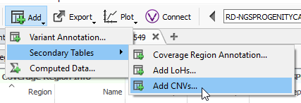
The final step for this part of the blog will be to run the CNV algorithm (Fig 16).
When setting up the CNV algorithm menu (Fig 17), the top portion shows two tabs (Parameters and Advanced), as well as the Sensitivity <–> Precision slider. If you slide the bar to sensitivity (Fig 18 a), and open the advanced tab, you’ll see that there is a specific probability level in place for three scenarios:
- Prior CNV probabilities
- Diploid to CNV transition
- CNV to CNV transitions
Likewise, if you slide the bar to precision (Fig 18 b), you’ll see probabilities are much smaller. Basically, this is a way for the user to control how many CNV are potentially discoverable. This is an important consideration for a user who is looking for new CNV findings. You may want to have a CNV run with high precision, as these CNVs would go beyond these strict probabilities and represent your calls with the strongest evidence. You can also have multiple CNV runs in a single project which allows you to do both a strict precision run and more open sensitive run to assess both scenarios.
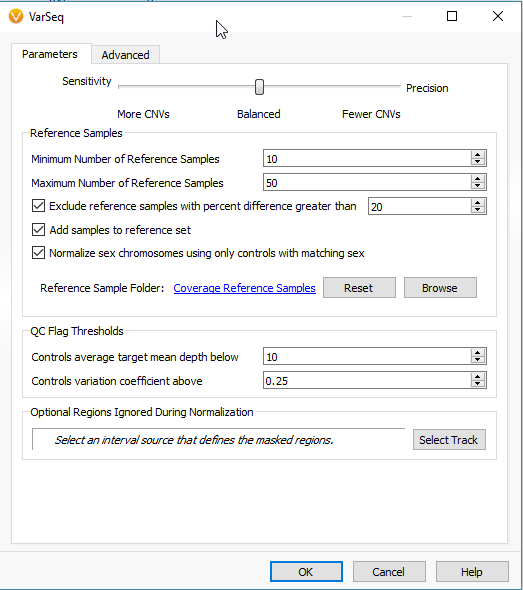


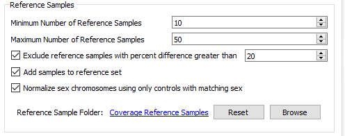
The next section of the menu is to modify the settings for your reference samples (Fig 19). From the reference sample set we built earlier, we can adjust the minimum and the maximum number of individual reference samples used for normalization. Not all reference samples get used for normalization; the algorithm will prioritize which references are most similar to each SOI in coverage profile. It is also critical to note that your reference samples should come from the same library prep method/platform. Essentially, the algorithm is going to do what it can to prevent comparing apples to oranges. However, the user should also prevent trying to detect events across a melting pot of sample data from multiple sources. Over time and the collection of numerous references, you may be more stringent on acceptable references for how much they differ from your SOI. The user can set a maximum acceptable percent difference but the default you will see is set at 20%.
There are more specific features you can customize for your CNV caller, but you may consider starting with the default setting for the first run since we have sought to optimize these defaults for best results. With all the settings in place, you can then select OK to run CNVs.
Step 5: Exploring the CNV results
With the completion of the CNV computation, you will now see a new table listing the results (Fig 20). This is a great transition into the next series of this CNV quality blog and will give the user time to run their CNV algorithm before deep diving into the search for high-quality events.
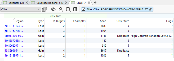
We will begin our next blog from this CNV table focusing on viewing high-quality CNVs specific to each sample, how to annotate against known/curated CNVs, and how the user can track reoccurring false/positive events building their own custom CNV annotation. I hope this blog aids our users when preparing their CNV projects. If issues arise or more questions are left unanswered, please do not hesitate to contact [email protected] for additional training.
This is a 2-part series on CNV setup & quality assessment – to read part 2, click here.


