First, thank you to everyone who joined us for our recent webcast, Handling a Variety of CNV Caller Inputs with VarSeq. Also, we would like to thank those that Tweeted #CNVsupport @GoldenHelix or emailed us ([email protected]) to throw in their questions. This was a successful trial run, and we would like to continue engaging with our users through these outlets. That aside, I would like to take you through a recap of some of our highlights and a few of our user-submitted questions concerning VS-CNV.
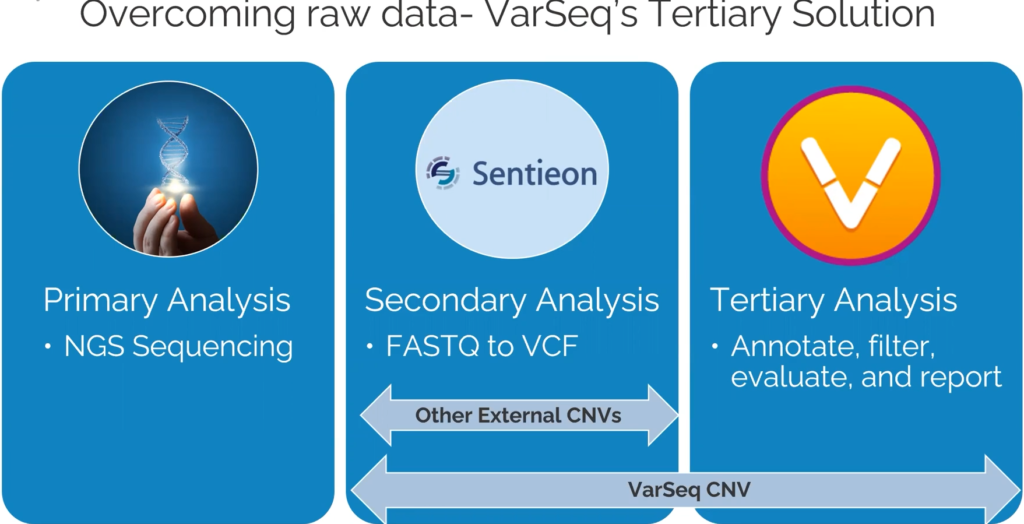
Let’s start off by defining VS-CNV (Figure 1). The VS-CNV program is a CNV caller and analysis platform all in one. Overcoming the challenges of basing CNV calls purely on read depth, VS-CNV develops a reference set from which VarSeq pulls the samples with the most similar coverage profile. In addition, there are metrics like the ratio, Z-score, and VAF that can be used to ensure there are high-quality calls. By spanning both the Secondary and Tertiary stages of NGS analysis, the VarSeq CNV caller has a high degree of clinically validated accuracy.
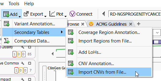
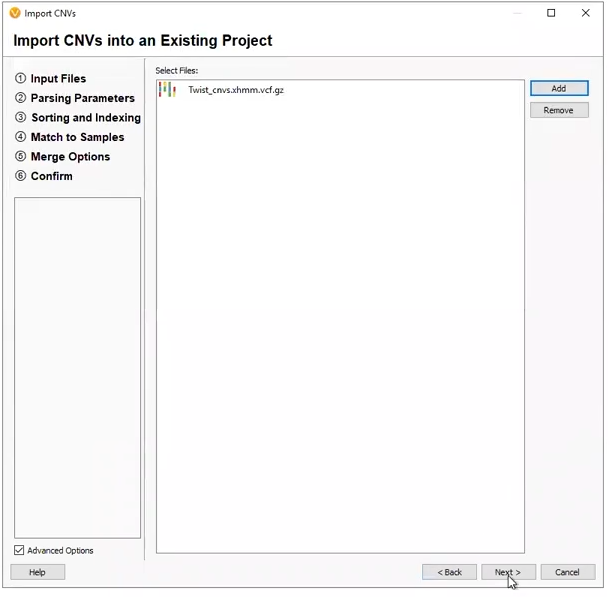
VarSeq CNV is not the only CNV caller around. Many different external callers will generate standard CNV VCFs. VarSeq CNV is not limited to CNVs called with the VarSeq software (Figure 2), and our development team has been working very hard to support all external CNV imports. The CNVs we can import include, and are not limited to, CNV VCFs from Dragen, XHMM, GATK, Delly, Manta, Lumpy, and of course, our own VS CNV. For licenses activated with VS-CNV, it is simply a matter of going to Add > Secondary Tables > and Import CNVs from File, to bring these data sources into the software.
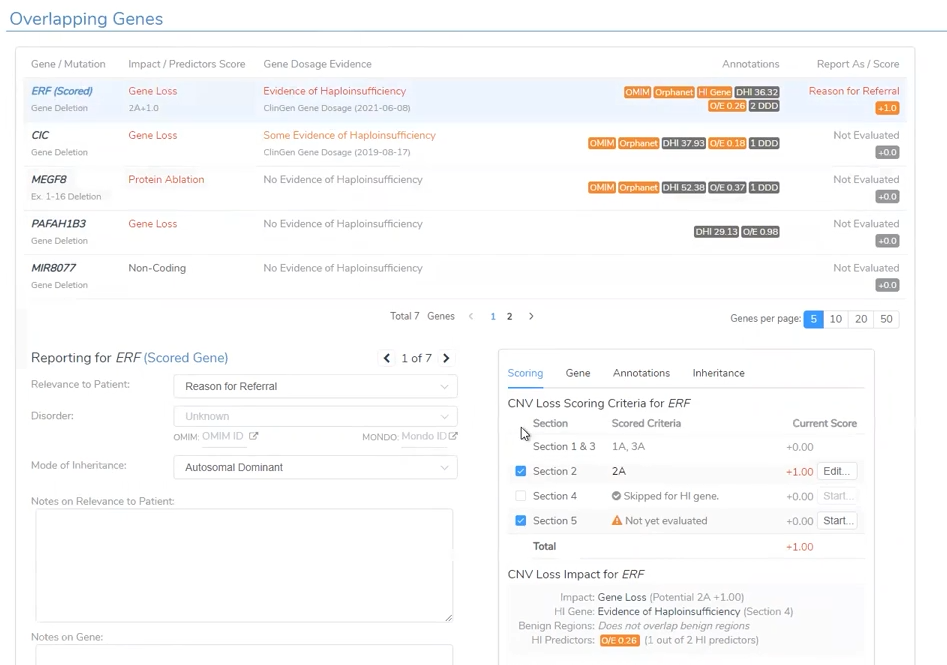
VarSeq CNV also supports the ACMG scoring for CNVs. The automatic scoring criteria are based on the Riggs et al., 2020, CNV scoring paper. This bases our CNV scoring on a sliding scale from -0.99 as Benign to +0.99 as a Pathogenic CNV (Figure 3). Scored inside of VSClinical, the accumulation of evidence for a Benign or Pathogenic CNV state will change the overall score and interpretation. Through VSClinical, these interpretations can be funneled into a final clinical report.
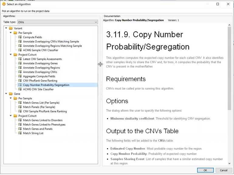
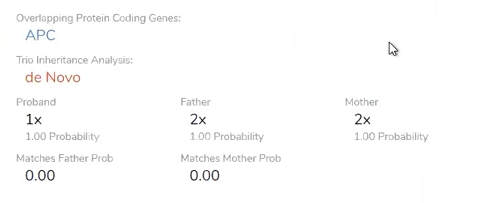
Through the webcast, we explored several flavors of CNV projects. Our first project was a Trio where CNVs had been called using VS-CNV. The Copy Number Probability and Segregation algorithm came into play here, allowing us to compare copy numbers in our proband versus the mother and father (Figure 4). This algorithm can only be applied to CNVs called with VS-CNV because it relies on the coverage regions to determine the similarity between samples.
The Copy Number Probability and Segregation Algorithm came into good use, as it helped us identify our CNV of interest as de novo in origin (Figure 5).
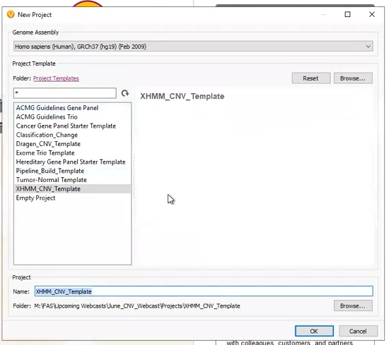
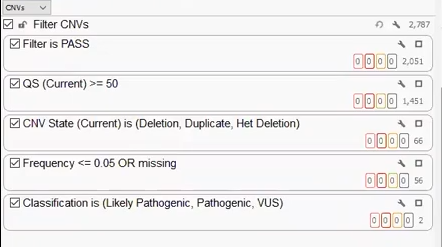
Our next two projects came from externally called CNVs. The first was a project derived from a pre-made template (Figure 6). This project was designed to work with an XHMM CNV VCF, with the filters premade, and the only work for the user to do was designate the variant VCF and CNV VCF (Figure 7).
Like the CNV analysis for the CNV called in the Trio project, VSClinical is able to take the user through the ACMG-based analysis with the automated scoring criteria (Figure 8). This project had a large Pathogenic CNV related to the Global Developmental Delay phenotype.
Our last project was created with a CNV VCF derived from Dragen. Like the other two projects, we can build a filter chain specific to the fields brought in on the VCF, isolating a handful of clinically relevant CNVs that can be brought into VSClinical for analysis (Figure 9).
We hope this webcast will highlight the VS-CNV flexibility through its support of many different CNV formats. After the webcast, some of our users reached out with additional questions that we would like to answer here.
One user asked us: How can we confirm the accuracy of the CNV caller in VarSeq?
As far as validation goes, every user will need to perform their own validation with the data from their own pipeline. This is the main reason Golden Helix cannot supply a shipped project template for all users, but as we saw in the webcast, you can create templates tailored to your workflow. You will want to consider some recommendations when setting up your CNV pipeline. For one, you will want to ensure that all samples come from the same library prep method. We don’t want to compare apples to oranges with samples from various kits and different callers. You will also want enough samples for ideal coverage that allows for normalization and averaging. Based on our internal testing, the best minimum reference sample count would be 30 or more.
Another user emailed us the question: Does my reference set need only to include true normals?
When using VS-CNV, you do not need to have true normals in the reference set for germline samples. The normalization process will adjust for any single sample’s loss, or increase of coverage. The exception here is somatic data, where you will want to ensure your reference set is composed of true normal germline samples. Moreover, be sure you have adequate coverage for the appropriate CNV method. This would include 100x average coverage for targeted regions, down to 1x coverage for binned regions on shallow whole genome data.
A viewer tweeted at us: @GoldenHelix does your CNV caller work with Amplicon data? #CNVsupport
CNV calling is not compatible with Amplicon data, so we advise you to keep that in mind while designing your experiments. Our VarSeq variant analysis, though, does support Amplicon data.
Another viewer tweeted: What size of CNVs can we expect to call with VarSeq? @GoldenHelix #CNVsupport
We deploy a probabilistic approach for smaller events, down to a single exon in size, then utilize segmentation to make the much larger calls at a whole chromosome level. VS-CNV is very flexible with the size of the detected CNVs.
And with that, thank you again to our viewers who reached out with their questions. If you have any other questions or want to learn more about VarSeq CNVs, please reach out to us at [email protected] or through Twitter at @GoldenHelix #CNVsupport.
