Since the initial release of the copy number variant algorithms in VarSeq, our team has created a variety of content to help users get started with building their copy number variant projects. In our webcast library, you can find a few of our recent webcasts in 2019 covering CNV workflows and validation:

• Clinical Validation of Copy Number Variants Using the AMP Guidelines
• CNV Annotations: a crucial step in your variant analysis
• Clinical Validation of Copy Number Variant Detection by Next-Gen Sequencing

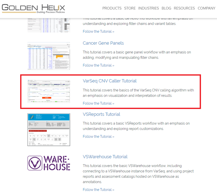
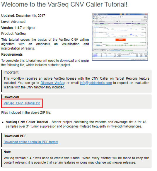
Or, if you prefer to take a more detailed, hands-on approach, you can look to our Tutorials for a step-by-step guide on how to start the CNV process (Figure 1). When you first open the VarSeq copy number variant Caller Tutorial you will find the project ‘VarSeq_CNV_Tutorial.zip’ file which you will need to download before getting started (Figure 2).

Please note that in order to access our tutorials, you will need an active VarSeq license with the CNV Caller on Target Regions feature. If you are interested in activating a free trial for this project, please email [email protected].

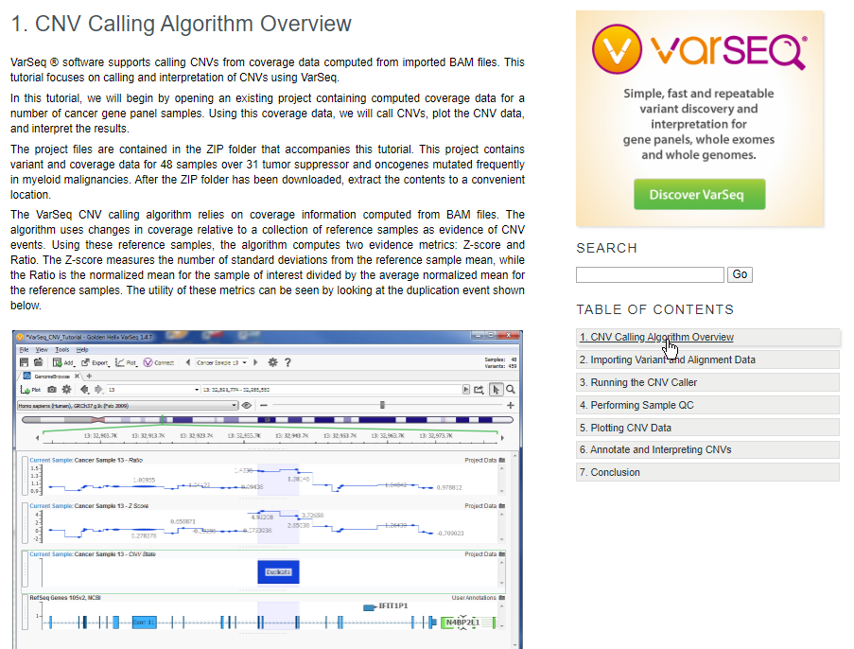
We recommend reading the Overview which will layout the framework for how CNVs are called using the coverage data in the sample BAM files and at which point the downloaded project will start the analysis (Figure 3).

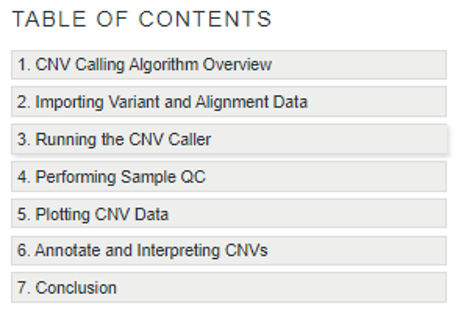
The Table of Contents (Figure 4) on the left side of the page will show each step of the process for the tutorial, beginning with importing data. This project will not require you to do any importing, but we wanted to describe the process of importing VCF and BAM files since many users follow the tutorial steps using their own data/projects. The project will begin with coverage statistics pre-calculated for each sample and the first step will be to compute CNVs. Following the Table of Contents, step 3 summarizes the options available when running the CNV caller which includes:

• Expected CNV Rate: The prior probability that a target is within a CNV event in the absence of evidence. A value of “Not Common” will result in fewer false positives but will increase the number of false negatives, while a value of “Common” will produce more false positives but will result in fewer false negatives.
• Minimum Number of Reference Samples: The minimum number of reference samples to be selected by the algorithm.
• Maximum Number of Reference Samples: The maximum number of reference samples to be selected by the algorithm.
• Exclude reference samples with percent difference greater than: This option will filter reference samples with a percent difference above the specified value after a minimum of 10 samples have been selected.
• Add samples to reference set: This option adds the current project’s sample to the set of reference samples.
• Independently normalize non-autosomal targets: If this option is selected, non-autosomal targets will not be normalized using the autosomal targets, but will instead be normalized separately. This option should be used if few non-autosomal targets are present, or if the entire X or Y chromosomes are likely to be deleted or duplicated.
• Controls average target mean depth below: Flags targets with average reference sample depth below the specified value.
• Controls variation coefficient above: Flags targets for which the variation coefficient is above the specified value. A high variation coefficient indicates that there is extreme variation in reference sample coverage for the target region.
• Optional Regions Ignored During Normalization: Here a region track ban be selected that provides coordinates for regions that will be excluded from the normalization process.

Once CNVs are computed, the next steps in the tutorial are to dig into the sample statistics to confirm the ideal sample quality which is critical to do before the evaluation of CNVs. Any sample that is low quality may warrant a “pause” on CNV analysis to first rerun the sample to improve the quality of coverage. Here are some examples of quality flags

• High IQR: High interquartile range for Z-score and ratio. This flag indicates that there is a high variance between targets for one or more of the evidence metrics.
• Low Sample Mean Depth: Sample mean depth below 30.
• Mismatch to reference samples: Match score indicates low similarity to control samples.
• Mismatch to non-autosomal reference samples: Match score indicates low similarity to non-autosomal control samples.
• Few Gender Matches: Not enough reference samples with matching gender to call X and Y CNVs.

If the sample quality checks out and no flags exist, then you ready for CNV analysis. The final two steps of the tutorial are to plot and annotate CNVs. Each of these annotations adds dramatic improvement in filtering the resulting CNVs to those clinically relevant to the patient. Obviously, there can be more complexity to this process and this tutorial only serves as an assist in getting started. If you would like more detailed training on the construction of your CNV project or post-discovery analysis, please reach out to [email protected] and we will be happy to help.