The table is set, the football game is on in the background, and the family has gathered around the table when out of nowhere, your Cousin Eddie shows up for Thanksgiving dinner. While Cousin Eddie is known for eating anything, his allergies always get the best of him, ruining the evening. Thankfully, this year Cousin Eddie had recently gotten his genome sequenced with PacBio HiFi long-read technology. Let’s delve into a workflow that takes advantage of our known phenotype, and allergies, and gets us down to relevant variants of interest.

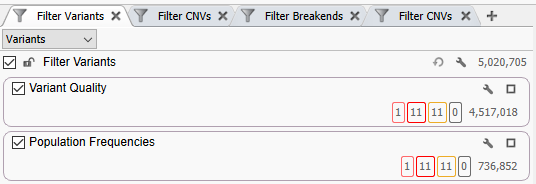
Like most of our standard workflows, we are starting with a Variant Quality container, and a Population Frequencies container (Figure 1). Although starting with more than five million variants may seem intimidating, with a good workflow design, we can easily get down to a handful of interesting variants. As you can see, most of these long-read calls are very high quality, as our Variant Quality container retains the majority of calls. For the Population Frequencies container, we are leveraging databases like 1kG Phase 3, GnomAD Genomes, TopMed, and more to retain variants that are otherwise ‘rare’ or ‘missing’ in healthy populations. As our phenotype of interest, allergies are fairly common, our filtering thresholds here may be much looser than if we were looking for a very rare disease. This container leaves us with over 700,000 high-quality and otherwise rare variant calls.

Next, we move into our Sequence Ontology container (Figure 2). The three open filters, Effect Combined, Predicted Novel Splice and Predicted Splicing Disrupted, are all derived from RefSeq. Here we are broadly looking for variants with a predictive disrupted function.

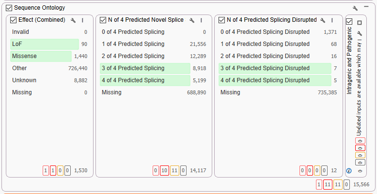
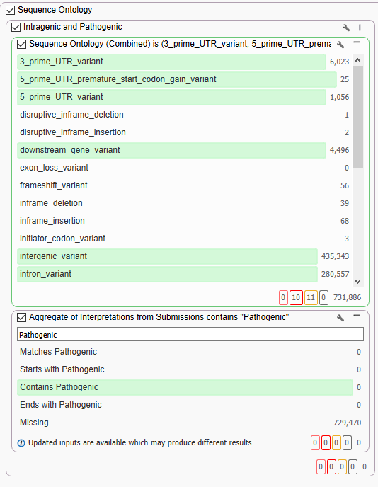
One of the big reasons to use long-read data, like the PacBio HiFi data, is to see all those deep intronic variants that can be missed with short-read technology. The figure above (Figure 2) had over 726,440 variants falling into the ‘other’ category that had no predicted function. The majority of those calls will be either synonymous or deep intronic variants. Now, there are a number of predictive tools and algorithms that could be applied to parse out more information on those calls, but for dear Cousin Eddie, we are just looking for probable pathogenic variants today. One combination of filters to achieve this goal is to couple Sequence Ontology for non-exon variants with a filter from ClinVar (Figure 3). Specifically, we are going to use the Aggregate of Interpretations from Submissions for any variant that has ever been classified as ‘Pathogenic,’ independent of review status. From here, we can see that of all those ‘other’ calls, none have ever been called pathogenic, and we can move on with our filter chain.

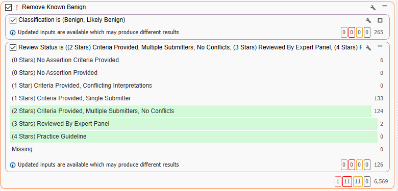
Using ClinVar once again (Figure 4), the goal is to now take variants that are called benign coupled with a high star review status. These are variants that have been reviewed by multiple sources with no conflicts for an overall call of benign. By inverting the container, we are ‘scrubbing’ out all of those well-defined benign variants.

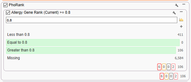
At this point, the filter chain can become fairly specific to our Cousin Eddie’s allergy phenotype. We can leverage PhoRank to prioritize variants in genes that are highly associated with the phenotype of ‘Allergy’ (Figure 5). If we had more specific phenotypes, for example, ‘milk allergy’ or any other phenotype, we could substitute that instead. This is a very effective filter as it reduces the number of variants down to 106.

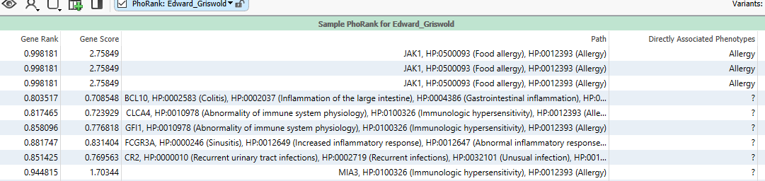
The term ‘allergy’ sits in a node with a great number of other phenotype connections. Looking at the figure below (Figure 6), we can see that some variants are in genes that are very closely associated to allergy. For example, the first row has a variant in JAK1, which is directly related to ‘food allergy,’ which is closely associated to ‘allergy.’ This is associated with a Gene Rank of over 99. Other variants are in genes that are less directly associated, for example, GFI1, which is associated with ‘abnormality of immune system physiology,’ which is associated with ‘immunologic hypersensitivity,’ which is then linked to ‘allergy.’ This longer thread of association means it has a lower score of 77. It becomes obvious that by fine-tuning the phenotypes entered, you can best find variants in genes that are related to a patient’s specific set of phenotypes.

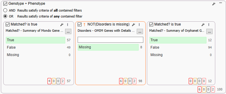
Although all the variants in genes that are related to allergy have made it through, because of the node-association system in PhoRank, it is possible to pull in variants in genes that themselves do not have well-defined OMIM or other summaries. Here we are leveraging Mondo, OMIM, and Orphanet databases to bring in variants that very specifically have those clinical phenotype or disorder breakdowns (Figure 7). Between the three databases, we are able to narrow our range to the final 100 variants.

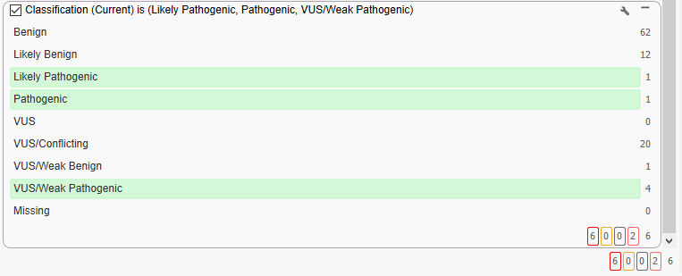
And finally, we are only interested in variants that are leaning towards Weak Pathogenic, or higher. In order to do this, we can bring in the VarSeq ACMG Auto-Classifier (Figure 8). This step is able to pull out those more Pathogenic variants, and so we see our final six.

The final six variants can be seen in the table below (Figure 9). While I have marked them all with the red ‘Primary Findings’ flag, take care to look at the two variants in the middle of the table that have the pink flag. What is interesting about these two is not only are they the only Pathogenic and Likely Pathogenic variants making it through the filter chain, but they are in the same gene, SPINK5. On top of that, we can see that, because of the HiFi long-read sequencing, we have phasing information that indicates they exist in trans, on opposite chromosomes. These two SPINK5 variants would be worth bringing into VSClinical for further analysis.

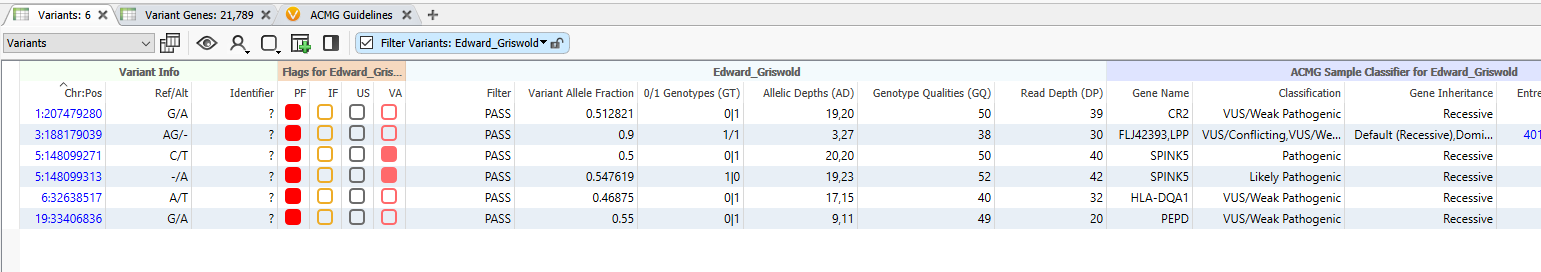
Overall, with a carefully constructed filter chain, we were able to go from an initial five million variants, down to a final six candidate variants. Those six variants are high-quality calls, with a strong association with our phenotype of interest, ‘allergy.’ In addition, because of the phasing information provided by the long-read sequencing, we can see that we have a Likely Pathogenic and Pathogenic variant existing in trans, one on each of Cousin Eddie’s chromosome five. If you would like to talk to us about your custom workflow needs, please reach out to us at support@goldenhelix.com. To our American customers who celebrate Thanksgiving, have a wonderful holiday!