With the release of our updated GWAS E-book, we have recently updated the GWAS example project (SNP Genome-Wide Association Tutorial – Complete). This updated project includes more details about how spreadsheets were generated, how to generate plots and which images were used for the GWAS E-book. This information can be found in the User Notes view in the project navigator and it will allow you to follow along with the SNP & Variation Suite (SVS) Viewer.

The SVS Viewer is available for free and allows you to view existing projects (spreadsheets and non-genomic plots) and visualize data in genomic contexts using GenomeBrowse. In this post we will walk through exploring the GWAS project with the SVS Viewer.

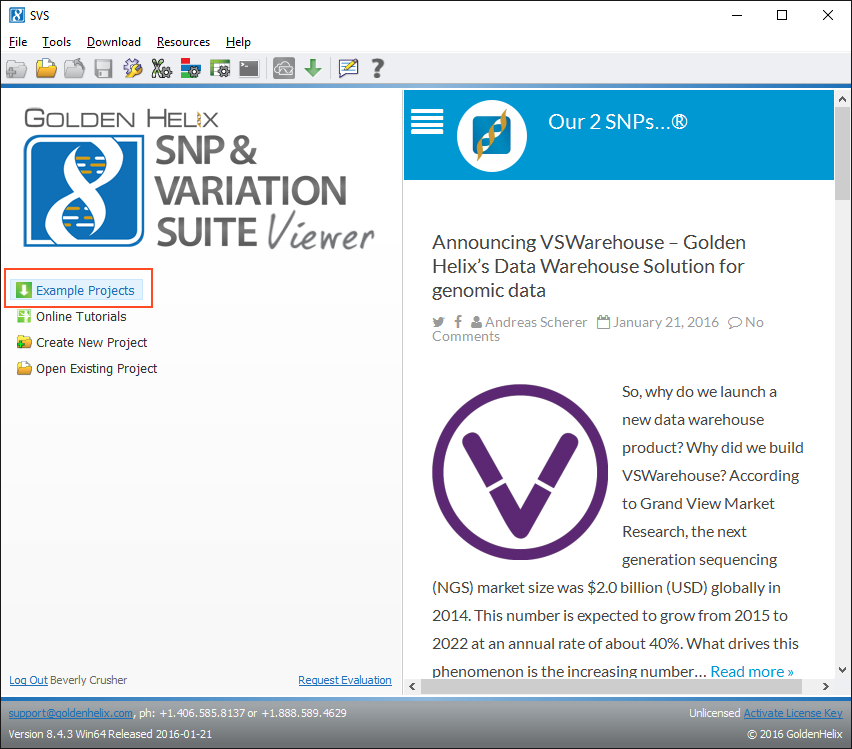
After downloading the SVS Viewer, download the Example Project by clicking on the Example Projects link or click on the Download menu and select Example Projects.

Fig. 1. SVS Viewer Welcome Screen

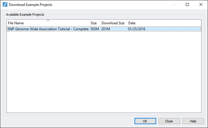
Select the SNP Genome-Wide Association Tutorial – Complete project from the list.

Fig. 2. Selecting the example project to download

Once the project is open it will contain the Navigator Window Nodes on the left, the Node Change Log and User Notes on the right. The User Notes will contain important information about how the data was created.

Fig. 3. SNP Genome-Wide Association Tutorial – Complete project navigator

You will notice that the nodes are color coded and those with a green flag indicate that the spreadsheet was used to create the Manhattan plot that was included in the GWAS E-book. As a reminder, only genomic plots can be created in viewer mode.

For example, open up the spreadsheet with the green flag (node 87). The spreadsheet should look like this:

Fig. 4. Association test results

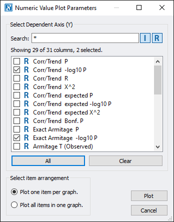
Now, go to GenomeBrowse and select Numeric Value Plot. Check both the Corr/Trend -log10 P and Exact Armitage Trend -log10 P boxes. Then click Plot. (Note: You may notice some grayed out options, which is normal as those options are only available in a licensed version of SVS.)

Fig. 5. Select values to plot in GenomeBrowse

Next, click on the Add button in the upper left-hand corner of GenomeBrowse and select both the COSMIC Mutations and DGV Variants sources from the Public Repository. Then click Plot and Close. The Add dialog should look like this:

Fig. 6. Select additional public data sources to plot in GenomeBrowse

Finally zoom into the region with our signal by copying this region: 6: 35,779,853 – 35,919,555 and pasting into the location bar.

Fig. 7. Final Manhattan results for the SRPK1 gene

To walk through the project yourself, you can download the SVS Viewer here. If you have any questions about this example project, please feel free to contact us at [email protected].