The ability to analyze copy number variants (CNVs) is an important aspect of any clinical or research workflow. While calling CNVs can be a challenging engineering problem, we are thrilled by our capacity to detect, analyze, and catalog CNVs all in the same place with VarSeq-CNV, our dedicated CNV analysis solution. In this blog, we will dive into the particulars of detecting CNVs with gene panel data. Elaborating on some specific details throughout the process will also shed light on the moving parts of the CNV algorithm.
Of course, calling CNVs is a nuanced process that requires expertise in evaluating the trade-offs of precision and accuracy. While we leave these decisions up to the user, we pride ourselves on our ability to provide thorough support and explanations of our tools. We are always available to provide one-on-one training and also have a number of blog and webcast resources.
While each of these resources provides practical information on using our CNV calling algorithm, we’d like to provide a guided overview here and shine some light on options that can optimize the algorithm for calling CNVs on smaller panels.
Preliminary steps for running the CNV caller
Current CNV users will be familiar with the steps outlined herein. Nonetheless, we’d like to reiterate the steps of calling CNVs in VarSeq and provide some general context as well as specific details in the gene panel paradigm.
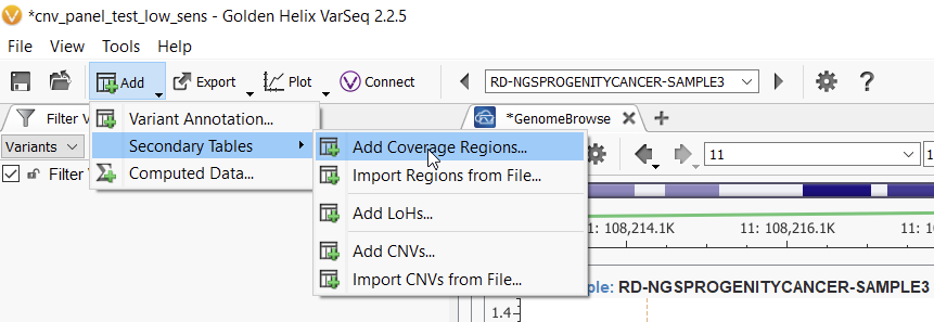
Assuming you have BAM files associated with the samples in your project, the first step to calling CNVs is running the Coverage Statistics Algorithm, which can be found in under Add > Secondary Tables > Add Coverage Regions (Figure 1).
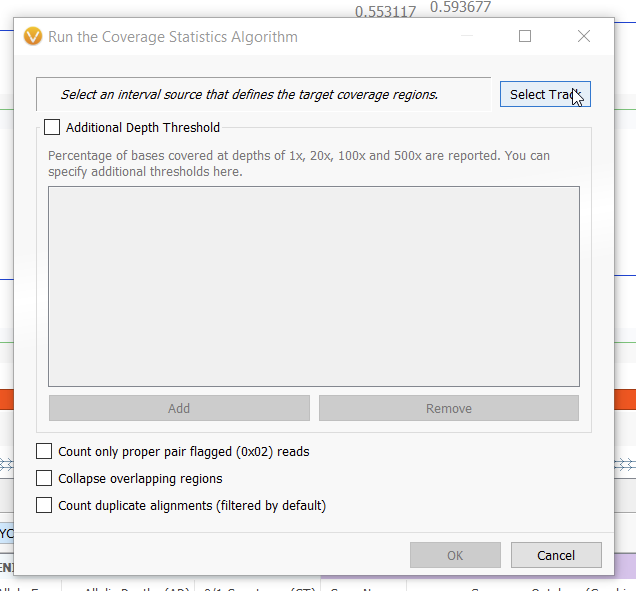
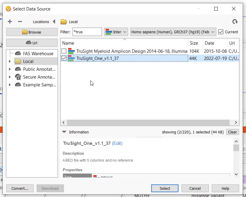
Selecting this option presents you with a dialogue box in which you must select an interval track that is derived from a BED file on which you want to calculate coverage statistics. If you have already converted a BED file to an interval track in the Data Source Manager, it will be available under local sources when you choose the Select Track option (Figure 2). In order to convert a BED file into an interval track, simply select Convert… in the bottom left of the next window (Figure 3) and follow the steps to convert BED file into a VarSeq-recognizable interval track, ensuring that you select the correct genome assembly. You can also input additional depth thresholds at which you’d like to calculate coverage in this window.
Another important component of the workflow to consider here is the breadth of the gene panels you are using. In the examples used below, we are using a gene panel with coverage in the range of 100 genes. Using too small a gene panel, for instance, 10 or fewer genes, is unlikely to provide enough coverage to accurately detect CNVs.
Once you have coverage regions run, the next step is to build your reference set to use in your CNV calculations.
Building a reference set
Our CNV algorithm functions by comparing the coverage over a given sample to the average coverage across a reference set of samples. There are two very important considerations here. The first is that the set of references and the sample being analyzed must be run through the same library preparation method. This is to ensure that the comparison of coverage actually remains as unbiased as possible. The second consideration is the somatic samples should not be used in the reference set; copy number variations are common and relatively unpredictable in tumor samples, and hence adding them to the reference will likely skew the results.
Beyond those two considerations, we recommend users have a reference set of at least 30 samples. Furthermore, as more samples are run through the aforementioned library preparation, they can and should be added to the reference set. This helps alleviate any unforeseen drift in sample statistics over time.
To add samples to the reference set prior to running the CNV algorithm, first, navigate to Tools > Manage Reference Set (Figure 4). If you’ve already added samples here, they’ll show up in a table with the Sample Name, Sample Checksum (basically a unique identified for each sample), Panel (the interval track associated with this reference set), and a Panel Hash (a unique identifier for the interval track) (Figure 5).


Needing to optimizing your caller?
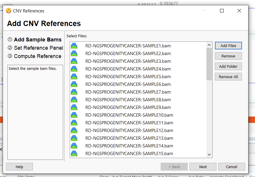
From here, we can add reference samples. It is essential that in doing so, we select the same converted BED file (now interval track) we used during our coverage statistics calculation. This is where the unique panel hash comes into play. Ensuring that you’re selecting the same panel, follow the steps of adding a BAM sample and selecting an interval track after clicking Add References (Figures 6, 7, and 8).


With our reference set correctly created, we can move on to the exciting part: calling CNVs. Here, we will outline the fundamental differences between calling CNVs on gene panel samples versus whole exome samples.
Calling CNVs with the appropriate settings
Most predictive algorithms have some sort of trade-off between sensitivity (related to the rate of false positives) and precision (related to the rate of false negatives), and our CNV caller is no different. We must strike a balance between ensuring that we’re bringing in relevant CNVs, and not overwhelming ourselves with dubious calls that need to be filtered out. This is where the options in the CNV caller come in. In the context of our walk-through, with coverage region statistics calculated and a reference set built, we can now call our CNVs. Navigating to Add > Secondary Tables > Add CNVs… will bring up a dialogue where we can set the parameters of the algorithm (Figures 9 and 10).

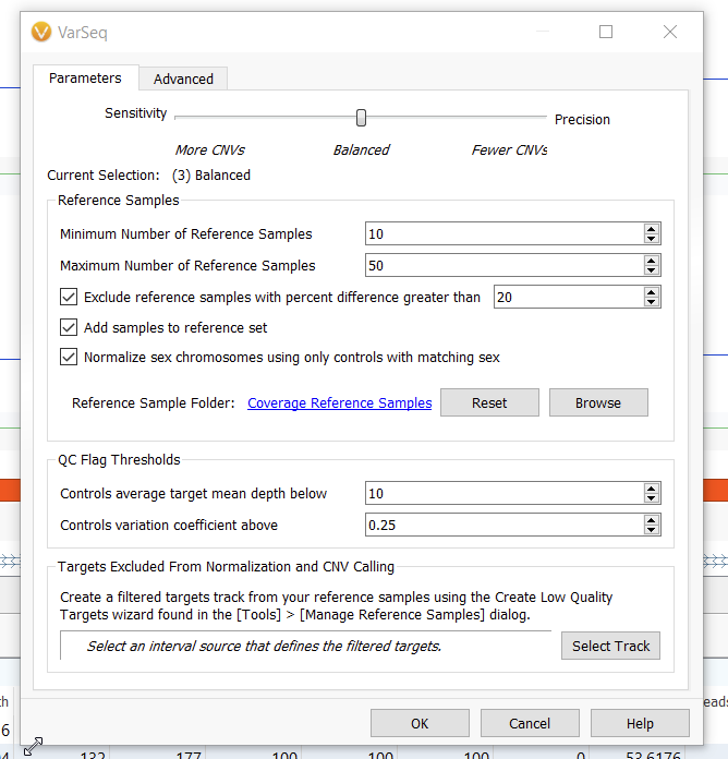
While sticking with the Balanced option is a great place to start for whole exome sequencing data, skewing more towards the Sensitivity end of the scale is often a better choice for panels. While exomes have a large breadth of regions over which to calculate the Z-scores and ratios we use in our CNV detection, gene panels have fewer loci over which to obtain these criteria. Hence, we tend to see data that doesn’t approach the same level of normalization and so can afford to be more sensitive.
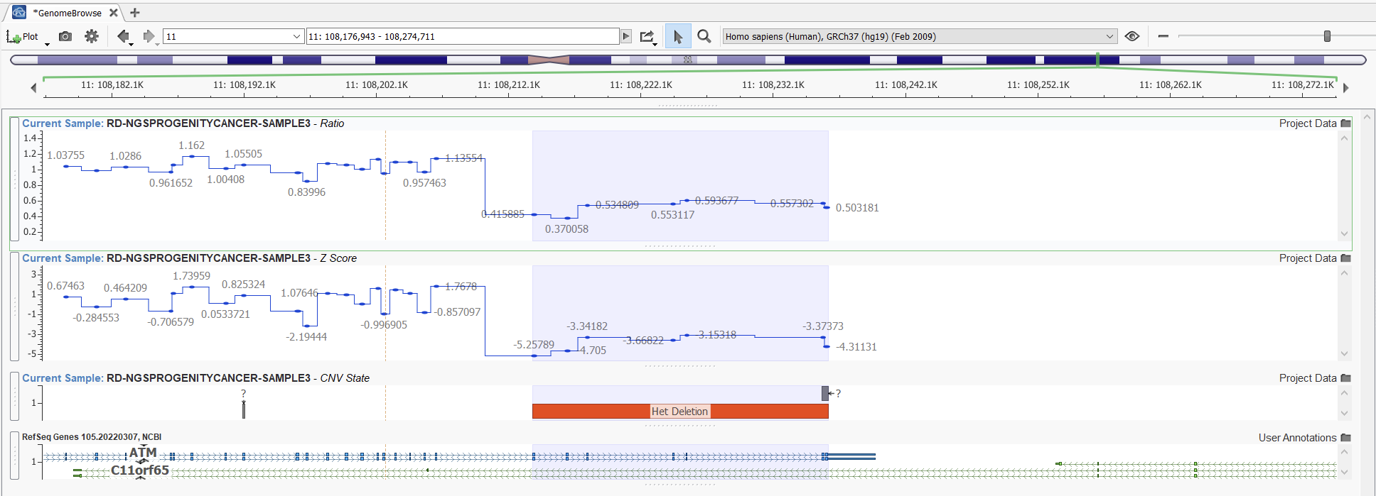
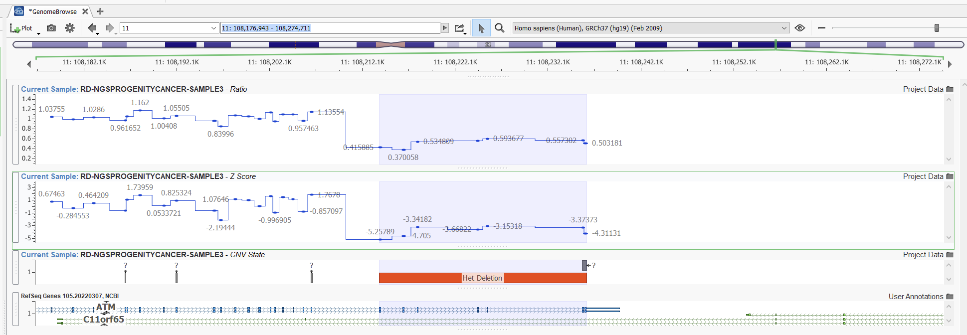
Let’s look at an example. Here we can compare two projects with the same samples and CNVs detected using the Balanced setting versus the Highest Sensitivity setting. Obvious CNVs, such as this heterozygous deletion with a consistent ratio of around 0.5, are picked up easily with both settings (Figures 11 and 12).
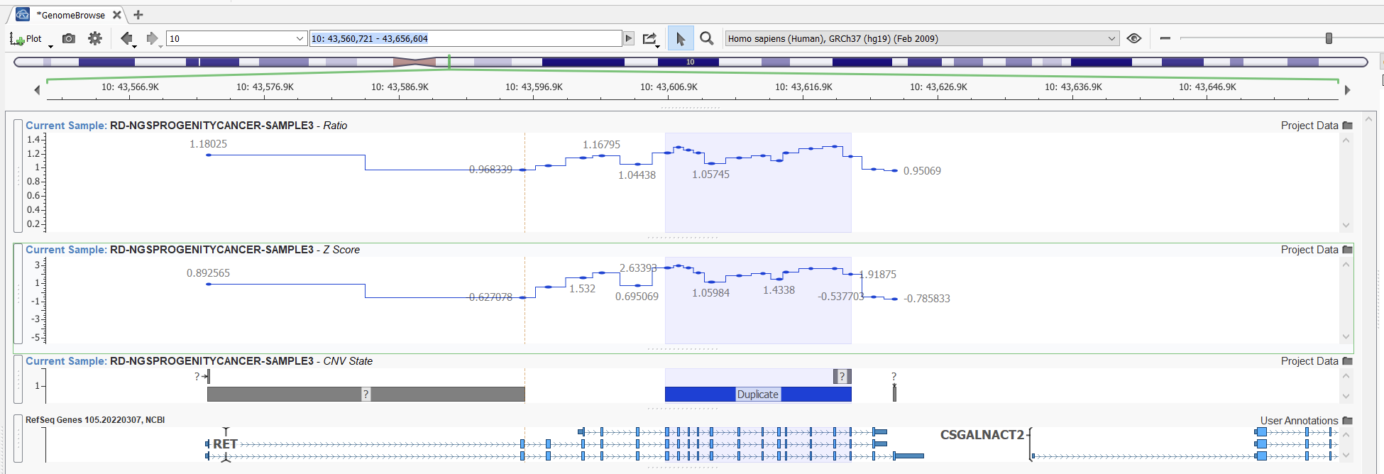
In this second example (Figures 13 and 14), however, we can see a case where our higher sensitivity project is picking up a fairly reputable duplication that our project with balanced sensitivity is missing. Looking at the ratio in this area, we can see that despite some noise, we see some reasonable elevations in ratio indicative of a duplication.

While this may yield unwieldy results in a whole exome project, in the case of gene panel projects, we can still be granular about how we identify high-quality CNV calls. In exome projects, increasing the sensitivity will produce more CNV calls in the order of thousands. By comparison, the order is closer to tens with increased CNV sensitivity in gene panels. Hence, using the higher sensitivity option is a great way to ensure the capture of all CNVs in gene panel projects.
In summary, we’ve reiterated the steps of calling CNVs in some detail and provided some tips on how to best optimize the CNV caller for gene panel projects. Of course, at the end of the day, we leave it to you to decide how to validate your CNV workflow. We also have some great additional reading and listening for users looking to learn more about our CNV caller.
Our webcast on calling CNVs for exome samples is a great resource for learning about different CNV use cases, and more information on analyzing CNVs using our automated ACMG guidelines is covered in this blog. We also dive into some more detail on algorithms associated with CNVs in this blog on CNV probability and inheritance, and interested users can also explore a detailed breakdown of our CNV calling algorithm in one of our first CNV blog posts. Lastly, please do not hesitate to reach out to us at [email protected] with any questions not addressed here.
Golden Helix has pioneered an industry-leading CNV calling algorithm that operates on existing clinical NGS gene panel, exome, and whole genome NGS data. Along with the calling of CNV events, the entire workflow is managed inside VarSeq’s clinical interpretation workflow. This integration enables CNV events to be considered alongside the annotated and filtered NGS small variants and incorporated into clinical reporting using VSReports.